2.1 The Cauchy–Riemann theorems

Here we will explore the relationship between complex differentiation and real differentiation. To do this, we introduce the notion of a partial derivative and use it to derive the Cauchy–Riemann equations (pronounced ‘coh-she ree-man’). These equations are conditions that any differentiable complex function must satisfy, so they can be used to test whether a given complex function is differentiable. In particular, we use them to investigate the differentiability of the complex exponential function. The technique is to split the exponential function

into its real and imaginary parts:

each of which is a real-valued function of the real variables  and . The derivative of exp is then calculated by using the derivatives of the real trigonometric and exponential functions, which we assume to be known.

Before we deal with the exponential function, however, let us first consider the simpler function . By writing , we see that

Let us define

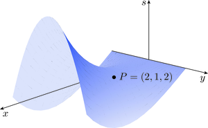
Then and are the real and imaginary parts of , respectively; that is, and . For the moment we will concentrate on the real part ; part of its graph (given by the equation ) is shown in Figure 9. Since is a function of two real variables, its graph is a surface. The height of the surface above the -plane represents the value of the function at the point . For instance, the point on the surface has coordinates because .

Figure 9 Graph of

Show description|Hide description

The figure consists of a perspective drawing of a three-dimensional set of Cartesian axes with a smooth surface sketched on it. The complex plane is drawn as horizontal, with axes labelled x and y. The x-axis points out of the page and to the left and the y-axis points out of the page and to the right from the origin. The vertical axis is labelled s. A smooth surface shaded darker on top and lighter underneath starts like a sheet with the top edge attached along the y-axis. At this point it is flat. As the x-coordinate increases, the surface rises up in a saddle shape above the x-axis, and dips down on either side. The vertical cross-section of the surface parallel to the s-y plane is shaped like an inverted parabola, symmetrical about a vertical line through the x-axis. On the surface a point is marked with a solid dot and labelled with its coordinates: capital P equals, open bracket, 2 comma 1 comma 2, close bracket.

Figure 9 Graph of

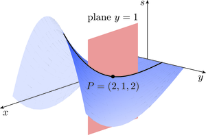
Let us now explore the concept of the gradient of the surface at a point such as . We will find that the answer depends on the ‘direction’ from which we approach the point. To make this more precise, consider Figure 10, in which the vertical plane with equation is shown intersecting the surface in a curve that passes through . By substituting into , we see that the curve has equation , so we can calculate its gradient at ; this is the gradient of the surface in the -direction at .

Figure 10 Intersection of the graph of with the vertical plane

Show description|Hide description

This figure is identical to Figure 9, except for the addition of a vertical plane, parallel to the x-axis and intersecting the curved surface. It consists of a perspective drawing of a three-dimensional set of Cartesian axes with a smooth surface sketched on it. The complex plane is drawn as horizontal, with axes labelled x and y. The x-axis points to the left and the y-axis to the right from the origin. The vertical axis is labelled s. A smooth surface shaded darker on top and lighter underneath starts like a sheet with the top edge attached along the y-axis. At this point it is flat. As the x-coordinate increases, the surface rises up in a saddle shape above the x-axis, and dips down on either side. The vertical cross-section of the surface parallel to the s-y plane is shaped like an inverted parabola, symmetrical about a vertical line through the x-axis. On the surface a point is marked with a solid dot and labelled with its coordinates: capital P equals, open bracket, 2 comma 1 comma 2, close bracket. The vertical plane is shaded red, and labelled with its equation, y equals 1. A curve is drawn on the surface to show where the surface intersects the plane. It passes through the point marked P.

Figure 10 Intersection of the graph of with the vertical plane

More generally, whenever we intersect the surface with a vertical plane with equation , we obtain a curve on the surface with equation (where is considered to be fixed). We can find the gradient at any point on this curve by differentiating with respect to and then substituting and . The resulting expression is called the partial derivative of with respect to at , and it is denoted by

A curly is used rather than a straight to emphasise that this is a partial derivative, for which we differentiate with respect to one variable and keep the other variable fixed. In our particular case, differentiating with respect to (and keeping fixed) gives

and substituting and gives

Hence the gradient of the surface in the -direction at the point is 9. This is a positive value because near the point , increases as increases (with ), as you can see from Figure 10.

Figure 11 shows the vertical plane with equation intersecting the surface in a different curve that passes through .

Figure 11 Intersection of the graph of with the vertical plane

Show description|Hide description

This figure is identical to Figure 9, except for the addition of a vertical plane, parallel to the y-axis and intersecting the curved surface. It consists of a perspective drawing of a three-dimensional set of Cartesian axes with a smooth surface sketched on it. The complex plane is drawn as horizontal, with axes labelled x and y. The x-axis points to the left and the y-axis to the right from the origin. The vertical axis is labelled s. A smooth surface shaded darker on top and lighter underneath starts like a sheet with the top edge attached along the y-axis. At this point it is flat. As the x-coordinate increases, the surface rises up in a saddle shape above the x-axis, and dips down on either side. The vertical cross-section of the surface parallel to the s-y plane is shaped like an inverted parabola, symmetrical about a vertical line through the x-axis. On the surface a point is marked with a solid dot and labelled with its coordinates: capital P equals, open bracket, 2 comma 1 comma 2, close bracket. The vertical plane is shaded red, and labelled with its equation, x equals 2. A curve is drawn on the surface to show where the surface intersects the plane. It passes through the point marked P.

Figure 11 Intersection of the graph of with the vertical plane

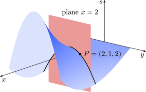
Reasoning similarly to before, we see that intersecting the surface with a vertical plane with equation gives a curve on the surface, and we can obtain the gradient at a point on this curve by differentiating with respect to while keeping fixed (and then substituting and ). The resulting expression is called the partial derivative of with respect to at , and it is denoted by

Differentiating with respect to (and keeping fixed) gives

this is the gradient of the surface in the -direction at the point . It is a negative value this time, because when and are positive, decreases as  increases (keeping fixed), as you can see from Figure 11.

You will need to work with partial derivatives a good deal here, so let us state the definitions formally.

Partial derivatives are real derivatives, not complex derivatives.

The next exercise asks you to work out the partial derivatives of the imaginary part of the complex function .

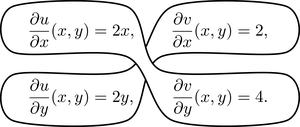
Let us collect together the partial derivatives of the real and imaginary parts and of the function :

As you can see, we have

This pair of equations is called the Cauchy–Riemann equations, and they hold true for the real and imaginary parts of any differentiable complex function, as the following important theorem testifies.

Origin of the Cauchy–Riemann equations

The Cauchy–Riemann equations are named after the mathematicians Augustin-Louis Cauchy and Bernhard Riemann (1826–1866), who were among the first to recognise the importance of these equations in complex analysis.

The Cauchy–Riemann equations first appeared in the work of another mathematician, however: the Frenchman Jean le Rond d’Alembert (1717–1783), who is perhaps best remembered for his work in classical mechanics. Indeed, the Cauchy–Riemann equations were written down by d’Alembert in an essay on fluid dynamics in 1752 to describe the velocity components of a two-dimensional irrotational fluid flow.

Jean le Rond d’Alembert (1717–1783)

Show description|Hide description

This figure shows the image of Jean le Rond d’Alembert. It is a head and shoulders shot with him looking to the right of the viewer.

Jean le Rond d’Alembert (1717–1783)

The Cauchy–Riemann Theorem gives us another strategy for proving the non-differentiability of a complex function. (Two other strategies were described earlier in Section 1.3.) If a complex function is differentiable, then it must satisfy the Cauchy–Riemann equations. So if those equations do not hold, then the function cannot be differentiable.

To illustrate this strategy, consider the function

The real part and imaginary part of this function are given by

Hence

Show description|Hide description

This figure shows the first partial derivatives of u and v with respect to x and y, shown in a two by two grid. Top left: partial derivative of u of x and y with respect to x equals two times x. Bottom left: partial derivative of u of x and y with respect to y equals two times y. Top right: partial derivative of v of x and y with respect to x equals two. Bottom right: partial derivative of v of x and y with respect to y equals four. The partial derivatives of u with respect to x and that of v with respect to y are grouped in a bubble, as are the partial derivatives of u with respect to y and that of v with respect to x.

As you can see, the partial derivatives have been grouped into two pairs according to the Cauchy–Riemann equations.

In this case, these equations are and , which are satisfied only when and ; that is, they are satisfied only when . If , then the Cauchy–Riemann equations fail, so Strategy C tells us that is not differentiable at .

Notice that the Cauchy–Riemann Theorem and Strategy C do not tell us whether is differentiable at the point at which the Cauchy–Riemann equations are satisfied. To deal with points of this type we need another theorem, which we will come to shortly. First, however, try the following exercise, to practise applying Strategy C.

We have seen that if the Cauchy–Riemann equations are not satisfied, then the function is not differentiable. Let us now describe an example to show that even if the Cauchy–Riemann equations are satisfied, then the function may still not be differentiable.

Consider the function , where for all and , and

The graph of is shown in Figure 12.

Figure 12 Graph of

Show description|Hide description

This figure consists of a perspective drawing of a three-dimensional set of Cartesian axes. The complex plane is drawn as horizontal, with axes labelled x and y. On the page, the x-axis slopes up and to the right in the positive direction, while the y-axis slopes up and to the left. The third axis is drawn as vertical on the page and is labelled s. It is used to represent the value of the real-valued function u, defined in the text, for each pair of values of x and y. The surface corresponding to the graph of the function u is shaded on the diagram. In the upper-left, lower-left and lower-right quadrants of the x-y plane, the function u takes the value zero, so the x y plane itself is shaded in these quadrants. In the upper-right quadrant, the value of the function at each point on the x-y plane is the minimum of the x and y coordinates of the point. The surface corresponding to the graph in the upper-right quadrant looks a little like a square pyramid, with the origin at one corner of its base, and one of its slant edges sloping up from the origin at an angle of 45 degrees, above the line y equals x on the x-y plane. To emphasise this shape, the slanting face of the pyramid that slopes up from the y-axis is shaded darker than the slanting face that slopes up from the x-axis.

Figure 12 Graph of

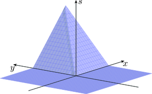
Since and take the value at all points on the - and -axes, we see that all the partial derivatives vanish at ; that is,

However, even though the Cauchy–Riemann equations are satisfied at the origin, is not differentiable there. To see this, observe that if , , then

whereas if , , then