2.2 Proof of the Cauchy–Riemann Converse Theorem

The proof of the Cauchy–Riemann Converse Theorem is rather involved and may require more than one reading.

We will need two results from real analysis. The first result is known as the Mean Value Theorem.

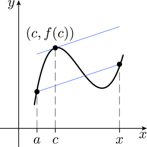
To appreciate why this theorem is true, imagine pushing the chord between and in Figure 13 parallel to itself until it becomes a tangent to the graph of at a point , where lies somewhere between and . Clearly, the gradient of the original chord must be equal to the gradient of the tangent, so

Multiplication by gives . Notice that this equation is also true if .

Figure 13 Graph of the real function

Show description|Hide description

This figure consists of a pair of Cartesian axes, labelled x and y. The diagram is focused on the upper-right quadrant. A curve representing part of the graph of an arbitrary real function f of x is drawn. (Actually, to facilitate the comprehensibility of the diagram, the graph is drawn to look like part of a cubic curve. It starts with positive gradient, then as x increases it reaches a local maximum, slopes down to a local minimum, and then slopes up again.) Three points are marked on the positive x-axis, labelled, from left to right, a, c and x. From each of these points a broken vertical line extends upwards to meet the curve. The three points where these three broken vertical lines meet the curve are marked with filled dots. The dot on the curve that lies above the point c on the x-axis is labelled with its coordinates, open bracket, c comma f of c, close bracket. This point is close to the local maximum of the graph. Through the point a line is drawn, tangent to the curve. A line segment is also drawn joining the other two points marked with dots on the curve (the points on the curve above the points a and x on the x-axis). This line segment is parallel to the tangent at c.

Figure 13 Graph of the real function

The second result that we will need is a Linear Approximation Theorem, which asserts that if is a real-valued function of two real variables and , then for near , the value of can be approximated by the value of the linear function defined by

Now, the graph of is a plane passing through the point on the graph of (Figure 14). Moreover, the partial - and -derivatives of coincide with the partial - and -derivatives of at . This means that both have the same gradient in the - and -directions, so you can think of the plane as the tangent plane to the graph of at .

Figure 14 Tangent plane to the graph of at the point

Show description|Hide description

The figure consists of a perspective drawing of a three-dimensional set of axes. The two axes in the horizontal plane are labelled x and y. The x-axis points out of the page and to the right; the y-axis points into the page and to the right. The vertical axis is labelled s. The diagram is focused on the section where x, y and s are all positive. The graph of the function u is shown as a convex curved surface shaded blue. The surface is labelled s equals u bracket x comma y close bracket. A point capital P is marked on the surface, and the tangent plane to the surface at the point capital P is shaded in red.

Figure 14 Tangent plane to the graph of at the point

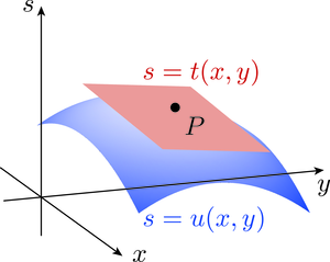
The accuracy with which this tangent plane approximates the graph of depends on the smoothness of the graph of . If the graph exhibits the kind of kink shown in Figure 12, then the approximation is not as good as for a function with continuous partial derivatives.

Since is the distance from to , the theorem asserts that the error function tends to zero ‘faster’ than this distance. Theorem 7 is the real-valued function analogue of Theorem 2.

Proof

We have to show that the function  defined by

satisfies

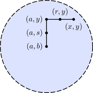
Since the partial derivatives exist on , they must be defined on some disc centred at . Let us begin by finding an expression for on this disc. If we apply the Mean Value Theorem to the real functions (where is kept constant) and , then we obtain

where is between and , and

where is between and (see Figure 15). Hence

Figure 15 Vertical and horizontal line segments from to

Show description|Hide description

The figure consists of a circle and two joined line segments. The centre of the circle is marked with a solid dot. This point is labelled with its coordinates, open bracket, a comma b, close bracket. A vertical line segment extends upwards from the centre of the circle, reaching about two-thirds of the way to the circumference. A point half-way up the line segment is marked with a solid dot, and labelled with its coordinates, open bracket, a comma s, close bracket. Another point at the top end of the vertical line segment is also marked with a solid dot, and labelled with its coordinates, open bracket, a comma y, close bracket. From this point at the top of the vertical line segment, a horizontal line segment extends to the right, reaching close to the circumference but remaining inside the circle. Half-way along it, a point is marked with a solid dot, and labelled with coordinates, open bracket, r comma y, close bracket. At the right-hand end of the horizontal line segment, a point is marked with a solid dot, and labelled with coordinates, open bracket, x comma y, close bracket.

Vertical and horizontal line segments from to

Substituting this expression for into the definition of , we obtain

Dividing both sides by , and noting that

(because both and do not exceed ), we see that

Figure 15 illustrates that as tends to , so do and . So, by the continuity of the partial - and -derivatives at , the two terms on the right of the inequality above must both tend to 0 as tends to . It follows that tends to 0 as tends to .∎

We are now in a position to prove the Cauchy–Riemann Converse Theorem.