1.1 Areas under curves

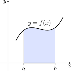
One of the uses of real integration is to determine the area under a curve. For example, the integral of a continuous function that takes only positive values between the real numbers and , where , is the area bounded by the graph of , the -axis, and the two vertical lines and , as illustrated by the shaded part of Figure 5.

Figure 5 Area under the graph of  between and 

Show description|Hide description

The figure shows the Cartesian axes labelled x and y concentrated in the upper-right quadrant. There is an arbitrary curve labelled y equals f of x contained inside the upper-right quadrant with one local maximum point and one local minimum point and the curve gradually rising bottom left to top right. There are points a and b marked on the positive x-axis with a being closer to the origin. These points are joined by a bold line. Vertical lines join the points a and b to the curve and the area between the curve and above the positive x-axis is shaded.

Figure 5 Area under the graph of  between and 

We can estimate this area by first splitting the interval into a finite number of subintervals, such as those shown in Figure 6.

Figure 6 Interval split into subintervals

Show description|Hide description

The figure shows a single horizontal axis labelled x. The points a and b are marked with a being on the left and b on the right. The interval a to b is split into five irregular subintervals. A horizontal brace is drawn beneath the axis and connects a and b; there is a label that says subintervals of open-square-bracket a comma b close-square-bracket.

Figure 6 Interval split into subintervals

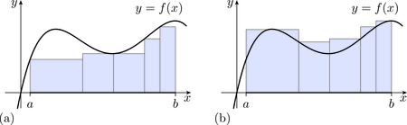
We can then underestimate the area under the graph of  between  and  by summing the areas of those rectangles that have the various subintervals as bases and for which the top edge of each rectangle touches the graph from below, as shown in Figure 7(a). Similarly, we can overestimate the area under between  and  by summing the areas of those rectangles that have the various subintervals as bases and for which the top edge of each rectangle touches the graph from above, as shown in Figure 7(b).

Figure 7 (a) An underestimate (b) An overestimate

Show description|Hide description

The figure is in two parts: (a) and (b). Each part shows a set of Cartesian axes labelled x and y and focuses on the upper-right quadrant. Both parts have the same curve labelled y equals f of x which is a curve going through the origin from the lower-left quadrant but concentrated mainly in the upper-right quadrant and it has two local maximum points and one local minimum. In both parts the points a and b are marked on the positive x-axis with a being nearer the origin. A bold line joins the points a and b. There are five irregular subintervals shown as rectangles and shaded. Part (a) has the top of each shaded rectangle touching the graph from below. Part (b) has the top of each shaded rectangle touching the graph from above.

Figure 7 (a) An underestimate (b) An overestimate

We now let the number of subintervals tend to infinity, in such a way that the lengths of the subintervals tend to zero. It can be shown that the underestimates and overestimates of the area tend to a common limit , written as

We call  the area under the graph of between and .

This underestimating and overestimating approach is often how Riemann integration is first introduced, and you may have seen it before. However, we encounter a problem if we try to generalise this particular approach to complex functions. Inequalities between complex numbers have no meaning, so it makes no sense to try to estimate complex numbers from ‘below’ or ‘above’. To get round this problem, we now outline a different approach to defining the integral of a real function – one that does generalise to complex functions.

Rather than underestimating and overestimating the area under the curve with rectangles, we choose a single point inside each subinterval and use this to construct a rectangle whose base is the subinterval, and whose height is the value of the function at the chosen point. The sum of the areas of these rectangles should then be an approximation to the area under the graph. As long as our function is continuous on the interval , then this modified approach (which does generalise to complex integrals) agrees with the underestimating and overestimating approach.

In this section we use this modified approach to give a formal definition of the Riemann integral, and then we summarise the main properties of the Riemann integral. We omit all proofs, which can be found in texts on real analysis.