

1.2 Spreadsheet formulas
There is one final activity in this section on spreadsheets, bringing all these ideas together.
Activity 3 Spreadsheet formulas
The formulas used in a spreadsheet are displayed as shown in Figure 3. Note that the asterisk (*) is the notation for multiplication used in spreadsheets and that all entries have been rounded to the closest penny. This example shows UK VAT, which was 20 per cent in 2014 (20 per cent as a decimal is 0.2).
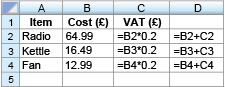
- a.The values in columns C and D will be displayed to two decimal places because they represent an amount of money. What values will be displayed in cells C3 and D3?
Answer
a.The formula in C3 is: (to 2 decimal places)
So,
The value in D3 is obtained by adding together the values in B3 and C3.
So,
- b.What do you think is being calculated in the cells in column D? Can you suggest a suitable heading for this column to be entered into D1?
Answer
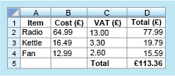
- b.Column D represents the total cost of the item plus VAT. A suitable heading might be ‘Total (£)’. You can think of other correct titles such as ‘Final Price (£)’.
- c.Cell D5 calculates the sum of the values in D2, D3 and D4. Write down a formula that could be entered in cell D5. What does this value represent?
Answer
c.The sum can be found by adding together the values in cells D2, D3 and D4. The formula ‘=D2+D3+D4’ could therefore be entered into cell D5. (Note that you do not use the formulas that are present in each of the cells you are adding. Just the cell title is sufficient.) Alternatively, you could use ‘SUM(D2:D4)’, which also adds together the cells from D2 to D4. The resulting entry represents the total cost (including VAT) of the radio, kettle and fan together.
With these changes, and the title ‘Total (£)’ typed into cell C5, the spreadsheet will look like the example shown here:
This section has served a few purposes. It has introduced spreadsheets and shown you how you can use these to carry out calculations as well as helping you make a start on writing your own formula. The next section leaves spreadsheets behind to continue with this latter skill, to build your confidence with formulas further.