

Linear graphs
In the video you saw an example of a linear (straight-line) graph (Figure 11).
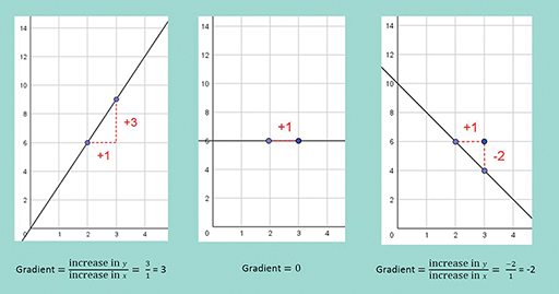
If a linear graph is increasing then its gradient is positive, since when increases by 1, y changes by a positive number. If a linear graph is decreasing, the gradient is a negative number.
What happens when the gradient of a linear graph is 0? The y-value does not change when increases and so the graph is horizontal.
Activity 8 Function detective
Recall the variables from Activity 7:
- age / number of hours of sleep
- number of people / how many chocolates each person gets
- sharing a box of 24 chocolates
- your age / your elder sibling’s age.
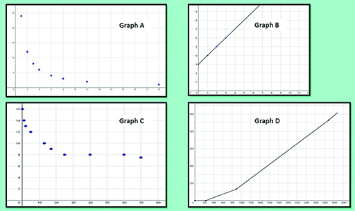
Match each pair with one of the graphs in Figure 12 below.
Is each graph increasing, decreasing or neither?
Discussion
Graph A
You should have found that graph A showed the relationship between the number of people sharing a box of 24 chocolates and how many chocolates each person gets. One way of checking this is to look for the points (1,24), (2, 12), (3, 8) that all lie on the graph. The graph is decreasing. Notice also that this graph is shown as a set of discrete points since the number of people and the number of chocolates are both discrete variables.
You could have chosen either variable for the x-axis (and the other for the y-axis) because this graph is the graph of a reciprocal function. The rule is that:
the number of people sharing a box of 24 chocolates x how many chocolates each person gets = 24
In symbols we could write that xy = 24
Or y = 24/x
Any function where y is a constant divided by x is a reciprocal function. A reciprocal function does not have a constant gradient since the slope changes along the graph.
Graph B
Graph B shows your age (on the x-axis) and (on the y-axis) the age of an (imaginary) sibling who was 3 years old when you are born. So it starts at (0,3). This point is called the y-intercept: it is the point where x takes the value zero. The graph is increasing. The gradient of the graph is 1 since your sibling’s age increases by 1 for every year you gain. The graph shows a linear function since it is a straight line with a constant gradient, but it is not a proportional relationship (see Week 3) because it does not start at (0,0). It is drawn as a line graph since age can be considered as a continuous variable.
Graph C
This graph is neither increasing or decreasing since there are intervals (between ages 20 and 60) in which the x-value increases but the y-value stays the same. It represents age on the x-axis and recommended hours of sleep on the y-axis. It only shows some data points, not joined by a line, so the variables are being treated as discrete variables. However, in the context we are clearly meant to use the data at the given ages to infer (make predictions about) the sleep needs at other ages.
It is unlikely that there is a simple mathematical function that will describe this graph.
Graph D
This graph is not one of those shown. It is an example of a piece-wise linear function, since the different sections are each straight lines. It shows weekly salary on the x-axis and how much income tax you pay on the y-axis (using the 2018-19 tax bands). The curriculum in England suggests that learners should be able to read information from graphs in financial contexts. Research suggests that it is necessary to discuss the context with learners before asking them to interpret graphs. Most 11-14 year olds would not be familiar with the idea that employers take tax out of your weekly pay.
So far we have met
- the linear graph which increases regularly so we can calculate a gradient. It has equation y = mx + c where m is the gradient and c is the (starting) value of y when x is zero. These graphs typically occur for costs, for travel or for conversion graphs are linear.
- the piece-wise linear graph which has straight line sections. It does not have a simple equation. These graphs occur when there are different types of cost or travel combined on one graph.
- the reciprocal graph with equation y = k/x .This graph typically occurs when sharing a constant amount k.
There is one final graph that we will meet in the next section.