

Introduction to differentiation
Introduction
This free OpenLearn course, Introduction to differentiation, is an extract from the Open University module MST124 Essential mathematics 1, an entry level module intended to provide a foundation in the essential mathematical ideas and techniques that underpin the study of mathematics and mathematical subjects such as physics, engineering and economics. MST124 looks at a variety of mathematical topics such as algebra, graphs, trigonometry, coordinate geometry, vectors, differentiation, integration, matrices, complex numbers and associated techniques. It also helps develop the abilities to study mathematics independently, to solve mathematical problems and to communicate mathematics. MST124 follows on naturally from the Open University module, MU123 Discovering mathematics.
Introduction to differentiation consists of material from MST124 Unit 6, Differentiation and has five sections in total. You should set aside between three to four hours to study each of the sections; the whole extract should take about 18 hours to study. The extract is a small part (around 8%) of a large module that is studied over eight months, and so can give only an approximate indication of the level and content of the full module.
The extract, which contains the first introduction to differentiation in MST124, is relatively self-contained and should be reasonably easy to understand for someone who has not studied any of the previous texts in the module. A few techniques and definitions taught in earlier units in MST124 are present in the extract without explanation, therefore a fluency with basic algebra and graphs is essential for this extract.
Introduction to differentiation
This course begins to introduce the fundamentally important topic of calculus. Calculus provides a way of solving many mathematical problems that can’t be solved using algebra alone. It’s the basis of essential mathematical models in areas such as science, engineering, economics and medicine, and is a fascinating topic in its own right.
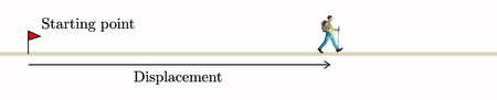
In essence, calculus allows you to work with situations where a quantity is continuously changing and its rate of change isn’t necessarily constant. As a simple example, imagine a man walking along a straight path, as shown in Figure 1. His displacement from his starting point changes continuously as he walks. The rate of change of displacement is called velocity.
Since the man’s displacement and velocity are along a straight line, they are one-dimensional vectors, and hence can be represented by scalars, with direction along the line indicated by the signs (plus or minus) of the scalars. Here we’ll work with displacement and velocity only along straight lines, and hence we’ll always represent these quantities by scalars.
If the man’s velocity is constant, then it’s straightforward to work with the relationship between the time that he’s been walking and his displacement from his starting point. You just use the equation
For example, if the man walks at a constant velocity of 6 kilometres per hour, then after two hours his displacement is
However, suppose that the man doesn’t walk at a constant velocity. For example, he might become more tired as he walks, and hence gradually slow down. Then the relationship between the time that he’s been walking and his displacement is more complicated. Calculus allows you to deal with relationships like this.
Calculus applies to all situations where one quantity changes smoothly with respect to another quantity. In the example above, the displacement of the walking man changes with respect to the time that he’s been walking. Similarly, the temperature in a metal rod with one end near a heat source changes with respect to the distance along the rod. Similarly again, the air pressure at a point in the Earth’s atmosphere changes with respect to the height of the point above the Earth’s surface, the concentration of a prescription drug in a patient’s bloodstream changes with respect to the time since the drug was administered, and the total cost of manufacturing many copies of a product changes with respect to the quantity of the product manufactured. You can see from the diversity of these examples just how widely applicable calculus is.
Basic calculus splits into two halves, known as differential calculus and integral calculus. (In this context ‘integral’ is pronounced with the emphasis on the ‘int’ rather than on the ‘eg’.) Roughly speaking, in differential calculus, you start off knowing the values taken by a changing quantity throughout a period of change, and you use this information to find the values taken by the rate of change of the quantity throughout the same period. For example, suppose that you’re interested in modelling the man’s walk as he gradually slows down. You might have worked out a formula that expresses his displacement at any moment during his walk in terms of the time that he’s been walking. Differential calculus allows you to use this information to deduce his velocity (his rate of change of displacement) at any moment during his walk.
In integral calculus, you carry out the opposite process to differential calculus. For example, suppose that you’ve modelled the man’s walk by finding a formula that expresses his velocity at any moment during his walk in terms of the time that he’s been walking. Integral calculus allows you to use this information to deduce his displacement at any moment during his walk.
Surprisingly, you can also use integral calculus to solve some types of problem that at first sight seem to have little connection with rates of change. For example, you can use it to find the exact area of a shape whose boundary is a curve or is made up of several curves.
Calculus
The name ‘calculus’ is actually a shortened version of the historical name given to the subject, which is ‘the calculus of infinitesimals’. The word ‘calculus’ just means a system of calculation. The word comes from Latin, in which ‘calculus’ means ‘stone’ – the link is in the use of stones for counting.
The calculus of infinitesimals became so overwhelmingly important compared to other types of calculus that the word ‘calculus’, used alone, is now always understood to refer to it.
An ‘infinitesimal’ was regarded as an infinitely small part of something. When you consider an object’s velocity, for example, in the calculus of infinitesimals, you don’t consider its average velocity over some period of time, but rather its ‘instantaneous velocity’ – the velocity that it has during an infinitely small interval of time.
Although the ideas behind calculus are explained in quite a lot of detail in this course many of the explanations aren’t as mathematically precise and rigorous as it’s possible to make them, and the proofs of some results and formulas aren’t given at all. For example, the idea of a limit of an expression is introduced, but this idea is described in an intuitive way: the course doesn’t give a precise mathematical definition.
The reason for this is that it’s quite complicated to make the ideas of calculus absolutely precise. At this stage it’s not appropriate for you to learn about how this can be done, because the necessary profusion of small details would make it harder for you to understand the main ideas. Instead, the precise mathematical ideas behind calculus are covered in the subject area known as real analysis. You might like to study this subject at a later time.
Newton and Leibniz
The fundamental ideas of calculus were developed in the 1600s, independently by Isaac Newton in England and Gottfried Wilhelm Leibniz in Germany. (‘Leibniz’ is pronounced as ‘Libe-nits’.) Neither Newton nor Leibniz made their ideas rigorous – this work was done later by other mathematicians. There’s more about Newton and Leibniz later in this course.