
3.6 Systems concepts: dynamic behaviour: control
A system does not usually behave in a random manner – its actions are governed in some way. This can be achieved by using the control models, either singly or in combination, shown in Figure 32(a) and (b). The feedback (or closed loop) control model in Figure 32(a) works as follows:
-
a feature of the output from the transformation process is monitored;
-
information regarding this is ‘fed back’ to a comparator process that compares the value of the feature with a predetermined ‘objective’ value;
-
if the value falls within the predetermined limits, no further action is taken;
-
if the value is outside the predetermined limits, a signal is sent to alter an input to the process in order to correct its operation.
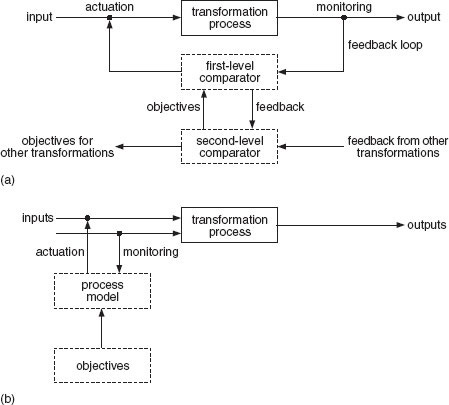
For example, suppose that the transformation process is drying in an oven. The objective is to maintain the temperature of the oven to within ±8 °C of a particular value. A sensor monitors the temperature of the oven. This is then compared with the preset limits, and corrective action is taken through an actuator if necessary. The important features of the model are as follows:
-
It repeats the basic structural pattern of input-process-output, with the addition of a feedback loop.
-
It shows two different levels of control: the first deals with feedback directly from the transformation process and the second with feedback from the lower level. This pattern of hierarchy of control is a feature of nearly all operations systems. The function of the higher level system is to provide standards for those at a lower level and to take corrective actions that are not within the competence of the lower level. The hierarchy is not, of course, restricted to two levels.
-
All or part of the output of the transformation process is monitored, either continuously or at intervals.
-
Information from the monitoring sensor is fed back to a comparator, which, as its name suggests, compares the value with a predetermined standard. If the value falls within the permitted range, no further action is taken. If the value is outside the limits, two courses of action are open. If the deviation can be corrected at that level of the system, an actuating signal is sent to alter one of the inputs to the process. If the deviation is outside the competence of this control level, the occurrence is reported to the higher level of control. The comparator may be a physical device (a microcomputer, for example), a person or a committee – though that would be rare at this level.
-
Actuation involves altering one of the inputs to the system to create the desired change in output.
The feedforward (or open loop) control model in Figure 32(b) is a control strategy used to correct or compensate for the variance of an input, to achieve a desired output variable. Feedforward can be used when the relationships between input, process and output are so well understood that it is possible to predict the effect of a particular change to an input. Feedforward control involves monitoring the condition of a critical input variable and predicting, using a model of the process, the effect that a variation will have on output.
This approach means that changes to the measured input or some other input variable can be made ‘before the event’. For example, suppose a strip is to be rolled to a thickness of 2 millimetres. The thickness of the incoming material could be monitored and roller pressure increased or decreased as necessary.
Particular attention has to be paid to the nature of the control parameters that are used as objectives in a control loop. For example, measuring machine hours and utilisation may, in the first instance, seem like a good idea. But if this results in the overproduction of components for stock it may be detrimental to the effectiveness of the system as a whole. This is another example of the importance of taking a holistic view.
The final concept associated with control is lag. This can be defined as the length of time that the control loop takes to correct an out-of-tolerance condition and can be expressed as:
The length of the lag in the control loop can have a significant influence on system performance. In a fully automated control system, total reaction time can be very small, but where clerical procedures are involved it may be lengthier.
Figure 33 shows an operations system consisting of five linked processes involved in the manufacture of printed circuit boards (PCBs) and the time (in seconds) that each operation takes.
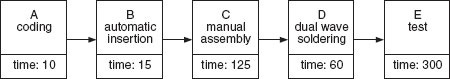
Each operation in Figure 33 involves:
A: Coding. The empty board is coded with part number and serial number.
B: Automatic insertion or mounting. Components are manually loaded and unloaded into an automatic mounting machine.
C: Manual assembly. Not all components can be mounted automatically. For example, block capacitors and switches have to be inserted into the PCB. The operator takes two boards and loads them into a carrier. The components are mounted. The fully populated board is mounted onto an in-feed conveyor that takes it through the soldering machine.
D: Soldering.
E: Testing.
The policy is to test one board fully every 10 minutes. In practice, depending on how busy the test technicians are with other work, the interval varies between 8 and 14 minutes, with the average at about 10 minutes. If a fault is detected, further tests are carried out to discover whether the problem is isolated or persistent. The corrective action taken depends on the type of fault and where it occurred. When problems occur with the settings on the automatic mounting machine they take about 10 minutes to correct from first detection during testing.
SAQ 12
If a fault occurs due to the settings on the automatic mounting machine, how long is the total mean control lag?
Answer
The mean control lag in seconds is calculated as follows:
| Automatic insertion | 15 | |
| Manual assembly | 125 | |
| Dual wave soldering | 60 | |
| Average monitoring internal | 600 | |
| Testing | 300 | |
| Time taken to correct settings | 600 | |
| Mean control lag | 1700 | ≈28 minutes |
At a rate of four boards a minute, this delay could represent 112 faulty PCBs.