

1.4 Boxplot activity 2
Activity 2 Boxplots of family sizes
The table below contains data on the sizes (numbers of children) of the completed families of two samples of mothers in Ontario. One sample of mothers had had fewer years of education than the other sample (six years or less for mothers in the first sample, and seven years or more for those in the other sample).
| Mother educated for six years or less |
| 14 13 4 14 10 2 13 5 0 0 13 3 9 2 10 11 13 5 14 |
| Mother educated for seven years or more |
| 0 4 0 2 3 3 0 4 7 1 9 4 3 2 3 2 16 6 0 13 6 6 5 9 10 5 4 3 3 5 2 3 5 15 5 |
Keyfitz, N. (1953) A factorial arrangement of comparisons of family size. American J. Sociology, 53, 470–480.
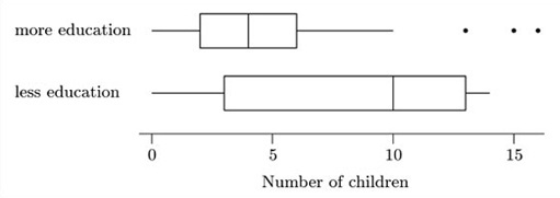
Comparative boxplots of the family size data are shown in Figure 1.7.
Compare the two samples of data using the systematic approach just outlined in the text. What conclusions can you draw about an association between education and family size?
Answer
Solution
Following the five steps for comparing boxplots outlined in the text, we begin with the medians (step 1). These are well separated, with the median for mothers with less education being higher at an astonishing 10. The length of the box for these mothers is more than twice that of the other box (step 2). The overall spreads (distances between adjacent values) are roughly similar for the two data sets (step 3). However, this comparison is perhaps less informative about dispersion than the comparison of box lengths, because of the potential outliers in the data set for mothers with more education. The overall range for mothers with more education is rather greater if these ‘outliers’ are included. However, if the untypicality of these values were to be seen as a reason for omitting them, the range for the mothers with less education would be the greater. Whether or not they are omitted, the difference in range is not huge.
The boxplot for mothers with less education shows some slight left-skew: the left whisker is longer than the right (step 4). The main body of data for the mothers with more years of education looks symmetric, but there are three large potential outliers which would undoubtedly have an effect on any calculations of skewness (step 5).
The two batches of data seem to be distributed differently in a way which is not merely the result of difference in location. The median for the mothers with less education is close to the upper adjacent value for the mothers with more education, which leads to the conclusion that the mother's education varies with family size. The main difference between the groups lies in their different concentrations around the median rather than their overall spread of values. The potential outliers for the mothers with more education are not very far from the upper adjacent value for the other sample, and are marked as outliers essentially because of the comparatively low interquartile range for the sample into which they fall.
The overall conclusion is that the mother's education does vary with family size, with those mothers receiving six or less years of formal education having, on average, larger families.
One thing the boxplots have also shown is that three data values in one of the samples are perhaps not typical; so calculations of the mean, standard deviation and skewness should be treated with certain amount of scepticism.