

9 Activities
Activity 1 Life cycle earnings
The New Earnings Survey publish various labour market statistics including the following information.
| Average gross weekly pay (in £) | ||
|---|---|---|
| Age | Females | Males |
| Under 18 | 125.2 | 127.8 |
| 18 to 20 | 160.9 | 180.7 |
| 21 to 24 | 218.8 | 263.8 |
| 25 to 29 | 281.5 | 331.8 |
| 30 to 39 | 320.1 | 405.8 |
| 40 to 49 | 301.2 | 445.8 |
| 50 to 49 | 272.5 | 420.5 |
| 60 to 64 | 236.0 | 341.3 |
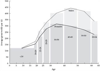
To what extent does the information in Table 8 support the view put forward in Section 5.3 that the age–earnings gap increases with age?
Answer
The general impression that can be seen from Table 8 is that female pay is less than male pay in all age ranges, although at under 18 this difference is negligible. Whether or not the gap between males and females increases, can be seen more clearly in Figure 5. This shows that male pay appears to grow until the 40–49 years age mark and then starts to decline, while female pay declines after the 30–39 years age band. Human capital theory predicts that women will earn less than men as they spend less active time in the labour market and are less likely to receive the same level of training and promotion opportunities. In Figure 5 female earnings range from 98 per cent of male earnings in the under 18 group to 65 per cent of male earnings in the 50–59 age range. In the 60–64 age range there is a slightly narrowing of the gap (69 per cent) as more males take retirement.
Caution needs to be taken here before making conclusive judgements, but it would suggest that a different profile in male and female life-time earnings does exist. It has to be recognised, however, that the data presented here is a snapshot and does not follow the same workers throughout their working lives. Nevertheless, the evidence would seem to support the view in the chapter that the gap between male and female pay generally widens as age increases.
Activity 2
Read the following statements and decide whether they would fit into the segmented labour market view. Explain your reasoning in each case.
An individual's productivity is the main determinant in his or her pay.
There is equal access and mobility for workers between sectors.
The labour market generates inequality in society rather than merely reflecting the inequality of that society.
The policy implications of segmented labour market theory include legislation and a more interventionist approach.
The labour market can only be explained by examining social and institutional factors affecting that market.
Answer
False.
Segmentation theorists would argue that it is the sector of the labour market in which individuals are employed that determines their pay and conditions. A neoclassical economist observing ‘bad’ jobs would be more likely to argue that such workers have less human capital, are less productive and therefore get less pay. Segmentation theorists would argue that the ‘bad’ jobs predominate in the secondary sector and a lack of training and investment in that sector keeps wages down.
False.
One characteristic of a segmented market is that mobility between sectors is limited. There will be movement within each sector but not across. Such factors as discrimination will strengthen the barriers to mobility.
True.
The argument here is based around whether the labour market, through market forces, reflects the fact that workers are unequal in their productive capacity and therefore earn different returns, or whether it is the labour market itself that generates inequality through dual markets. The segmented market approach sees the labour market as treating primary and secondary sector labour unequally. Returns to labour do not reflect potential productivity but actually limit such potential in the secondary market.
True.
The policy implications for a neoclassical economist is that workers on lower pay need to increase their human capital, thereby increasing their returns for companies. Educational and training reforms would be paramount to this viewpoint. Segmentation theorists would press more for legislation and intervention in the market place such as antidiscrimination policy. There would also be an acceptance of the role of trade unions in bargaining for workers in the secondary sector.
True.
The segmented theorist would put forward the view that it is impossible to explain the behaviour of the labour market in relation to the rewards of individuals in it without taking social and institutional factors into consideration. Neoclassical economists would probably state that such factors can be incorporated into their own framework.
Activity 3
This activity examines evidence on three hypothetical labour markets. You will need to both interpret what is being shown by the graphs and then in turn show how they apply to the theory of segmentation.

Examine the three distributions of earnings as shown in Figure 6 overleaf. Which of these (if any) could be argued to be supportive of a dual labour market? Explain your reasoning.
Answer
An examination of the three markets in Figure 6 would suggest that (b) and (c) are segmented markets. (b) is an example of strict duality where two clearly defined sectors are evident. It is clear that the primary sector with the ‘better’ high earning jobs is separate from the other jobs of the secondary market. Note that since annual earnings are considered, the often part-time, casual nature of work in the secondary labour market will be reflected in these frequencies.
(c) could be described as having ‘heuristic’ duality where a case could be made that while there is no strict duality, there is a spectrum of what could be described as ‘good’ and ‘bad’ jobs. Market (a) with uni-modality and a relatively small dispersion would suggest a competitive market.
Activity 4
This activity gets you to think through the various theories you have examined and apply them to a particular article.
Read the following article and answer the questions that follow.
HOW TO ISOLATE THE RACIST EMPLOYER: SIMPLISTIC ECONOMIC THEORY GIVES FALSE HOPE TO BRITAIN'S MINORITY ETHNIC GROUPS
Minority ethnic groups form a small but growing proportion of Britain's 58m population. From 4 per cent in the 1970s, their share rose to 5 per cent in the late 1980s and it should stabilise eventually at almost double that level.
As these relatively young communities come to be integrated more fully into the labour market it has often been assumed that the economic disadvantage they suffer relative to the majority white population should gradually erode. But recent trends suggest not.
Monority ethnic groups in the UK labour market
| Hourly earnings (£) | Employed % | Unemployed % | Inactive % | |
|---|---|---|---|---|
| White | 7.44 | 58 | 5 | 37 |
| All ethnic | 6.82 | 50 | 10 | 40 |
| Black | 6.92 | 53 | 13 | 34 |
| Indian | 6.70 | 59 | 8 | 33 |
| Pakistani/Bangladeshi | 5.39 | 32 | 11 | 57 |
According to the annual General Household Survey, the labour market position of blacks deteriorated relative to that of whites between the 1970s and 1980s. The difference between the black and white wage rose from 7.3 to 12.1 per cent while the difference between unemployment rates rose from 2.6 to 10.9 percentage points.
And things have got worse in the last few years. During the 1980s and early 1990s the unemployment rates of the minority ethnic groups behaved ‘super cyclically’ which is to say they did worse than the rest of the population when the economy was doing badly and better when it was doing well. […]
Identifying the source of ethnic differences in labour market performance is no easy task. A typical approach is to look at the differences in such factors as age, education, work experience, job description and type of employer. Any residual wage gap is assumed to be the result of ‘discrimination’.
Nobel prize winner Kenneth Arrow, defined discrimination in this sense as ‘the valuation in the market place of personal characteristics of the worker that are unrelated to productivity’. The major flaw with this approach – aside from the inevitable measurement difficulties – is that discrimination may also play an important part in determining people's productivity by affecting their access to educational opportunities.
The analysis is further confused by the fact that differences between circumstances of the various minority communities can be bigger than the differences between the minority ethnic groups as a whole and the white population. Nonetheless it is clear from everyday experience that discrimination remains a pervasive influence. So what could or should be done?
Imagine that a racist employer would not take on any ethnic minority workers because he believed them lazy, less intelligent or less dependable than their white counterparts. In the looking-glass world of simplistic economic theory these attitudes would receive their just desserts. Enlightened employers would attract the best ethnic minority candidates, boosting their productivity and allowing them to undercut racist employers and drive them out of the market.
Howard Davies, the deputy governor of the Bank of England therefore concluded in a recent speech to the Equal Opportunities Commission that one policy response should be to take a tougher attitude towards monopolies.
But while there are many good reasons to promote competition this may not be one of them. Predicting a would-be employee's potential productivity is expensive, time consuming and inherently uncertain. If an employer discerns that the productivity of whites is, on average, higher than that of blacks – say because of educational differences – then he or she may use race as a low-cost screening method.
This is clearly undesirable ex post if a high quality black candidate is passed over in favour of low-quality white. But in a world of incomplete information it may be an entirely rational way ex ante for an employer to maximize his profits. If that were the case then tougher competition might actually encourage discrimination.
This same uncertainty about individual productivity also makes it problematic to simply legislate against discrimination, because it is difficult to prove it is taking place. From a libertarian perspective, one might also argue that however distasteful it is to right-thinking people that employers, co-workers and customers discriminate against minority ethnic groups, that is not sufficient reason to legislate against it if falls short of racial hatred.
The best way to tackle racial disadvantage in the labour market may therefore be to concentrate on areas such as education. Studies in the US have traditionally concluded that between 30 and 50 per cent of the black–white wage gap is the result of discrimination. But Derek Neal of Chicago University and William Johnson of Virginia University argued last year that most of this residual in fact reflects a skill gap which can in turn be traced at least in part to observable differences in the family backgrounds and school environments of black and white children.
In Britain the proportion of 16–24 year olds from minority ethnic groups in full-time education is already more than half as a high as the proportion of whites. Pressing home this advantage would probably be a more effective policy response than relying on competitive pressures or legalistic regulations.
Source: Robert Chote, Financial Times, 17 June 1996
To what extent does the table in the article suggest that minority ethnic groups are disadvantaged in the labour market?
Critically assess the policy advocated by Howard Davies (’… a tougher attitude towards monopolies’) to reduce discrimination in the labour market.
Answer
From the table in the article it can be seen that in terms of earnings white workers have a considerable advantage. Across the different ethnic groupings workers in the Pakistani and Bangladeshi community have the lowest average earnings at £5.39 compared to £7.44 among white workers. In terms of employment rates, Indian workers with 59 per cent employment is higher than the black population with 53 per cent, but Indian workers’ hourly earnings are less than those for black workers. Only 32 per cent of those of Pakistani and Bangladeshi origin are employed with hourly earnings of £5.39 being the lowest of all ethnic groups. Overall a clear picture emerges of white workers faring considerably better in the labour market compared to minority ethnic groups.
Howard Davies’ policy proposal is in line with the neoclassical theory of Becker (see Section 5.2). Becker's model assumes competition will drive out the discriminating employer as their profits are reduced. The article describes a ‘looking-glass world of simplistic economic theory’ and how enlightened employers would realise that they could undercut rivals by employing quality workers from minority ethnic groups. The analysis would suggest that the discriminating firm will be forsaking profit to those firms who are non-discriminating. Such firms would be forced to leave the market as they begin to make losses.
However, if workers are faced with a dual market some will find themselves in a secondary market with poor conditions and pay that is not directly determined by their levels of productivity. They will find it difficult to move away from these ‘bad’ jobs and into the primary sector where better jobs exist and a more interventionist policy would be needed. Discrimination may be so endemic to the two-tier labour market that opening up competition will not be sufficient to overcome the problem. The severity of this institutional constraint is perhaps evidenced by the high proportions of people from minority ethnic groups who attend full-time education but are unable to break into the primary sector.
Activity 5
Table 10 shows a wage equation estimated by Kuhn (1987) using a sample of workers taken from the Canadian ‘Quality of Life’ Survey. The dependent variable, (log) hourly wages, is regressed on various individual characteristics, such as the age, education and union membership of the sample of workers. The sample contains persons who normally work at least 20 hours a week and are over 18 years of age.
Interpreting the results in the table, are women discriminated against in comparison to men in the Canadian labour market?
(Hint: Take a look at the wage equations earlier in the course: statistical discrimination (Section 5.3) and empirical analysis sections (Section 5.4).
| Men Coefficient | Women Coefficient | ||
| Intercept | 1.260 (11.455) | 1.165 (9.708) | |
| Age | 25–34 | .095 (1.792) | .116 (2.275) |
| 35–44 | .227 (3.661) | .156 (2.557) | |
| 45–54 | .195 (2.955) | .024 (0.375) | |
| 55–64 | .180 (2.571) | .024 (0.279) | |
| 65–76 | –.607 (–3.866) | –.190 (–0.848) | |
| Education | 8 years | .017 (0.193) | –.156 (–1.405) |
| 9–11 years | .216 (2.769) | .064 (0.667) | |
| 12 years | .274 (3.425) | .175 (1.882) | |
| 13–15 years | .420 (5.000) | .267 (2.697) | |
| 16 years | .613 (6.888) | .539 (5.233) | |
| 17+ years | .655 (7.043) | .581 (4.611) | |
| Tenure with current employer | 1 year | .050 (0.588) | .138 (1.747) |
| 2–3 years | –.008 (–0.101) | .132 (1.760) | |
| 4–5 years | .175 (2.134) | .144 (1.714) | |
| 6–10 years | .153 (1.866) | .253 (3.163) | |
| 11–20 years | .241 (2.869) | .424 (4.930) | |
| 21+ years | .287 (3.154) | .401 (3.457) | |
| Previous experience dummy | .059 (1.553) | –.061 (–1.564) | |
| Technical school | .071 (1.127) | .017 (0.266) | |
| Union membership | .089 (2.697) | .112 (2.800) | |
| Physical disability | –.022 (0.550) | .060 (1.333) | |
| Number of observations | 658 | 448 | |
| R2 | .246 | .309 |
Footnotes
t statistics are shown in bracketsAnswer
To discuss the evidence provided in Table 10 we need to compare both the size and sign of the coefficients, and their statistical significance. Consider first the coefficients for age, which provide a proxy for the human capital accumulated by workers as they get older. The coefficient 0.227 shows that for Canadian men the return from being aged between 35 and 44 in terms of the (log) wage received is 0.227. Compare this with the return of 0.156 for Canadian women in this age group. This particular comparison shows that there is discrimination because the return for women is less than the return for men for the same amount of human capital. Women also fare worse for ages 45 to 54 and between 55 and 64, where the coefficients are 0.195 and 0.180 for men, and 0.024 and 0.024 for women. Note, however, that for the 25 to 34 age group, the coefficient for women is larger at 0.116 than the 0.095 for men.
These comparisons should also take into account the statistical significance of each coefficient. We need to make a decision as to whether a coefficient is statistically different from zero, or in the formal language, whether the null hypothesis H0, that the coefficient is zero, can be rejected. Since for both men and women the number of observations are easily above 29, the critical value is for infinite degrees of freedom. For a two-tailed test at the 5 per cent level, the critical value is therefore 1.96. Under a two-tailed test, the alternative hypothesis Ha is that the coefficient is either more or less than zero. If we were carrying out a test at, say, the 10 per cent level of significance the critical value would be 1.645.
Looking at Table 10, we need to compare the t statistics, which are shown in brackets, with the critical value of 1.96. For example, the coefficient for men aged between 45 and 54 has a t statistic of 2.955. Since 2.955 > 1.96, the null hypothesis is rejected which means that the coefficient 0.195 is statistically significant from zero at the 5 per cent level.
Note that for this 45 to 54 age group, the t statistic for women is only 0.375. Since 0.375<1.96, the null hypothesis is accepted at the 5 per cent level – the coefficient is not significantly different from zero. This further exaggerates the extent of the discrimination in relation to this particular variable: since the return on age is now found to be 0.195 for men and zero for women.
For some of the other variables in the table, women get a higher return for their human capital than men. For example, consider the variable for 6 to 10 years tenure with current employer. The female coefficient of 0.253 is significant to the 5 per cent level since the t statistic 3.163 is more than the critical value of 1.96. But the t statistic for the male coefficient is 1.866 which is less than the critical value of 1.96. This means that the male coefficient is not significantly different from zero at the 5 per cent level while the female coefficient is statistically significant. Women earn more for this amount of tenure than men. They also earn more for tenure of between 11 to 20 years and for 21+ years, although in these cases the male coefficients are statistically significant.
To test for discrimination more formally, the decomposition method introduced in Section 5.4 would have to be followed. However, the insights drawn from Table 10 in the discussion above show that the evidence for discrimination against women is inconclusive, since the human capital coefficients are larger for women than for men for some of the variables given in the table.