

2.3 Financial feasibility
Before investment of resources in selecting and carrying out a potential project can proceed, two sets of questions need to be considered:
- Will the investment of resources in a particular project be worthwhile when compared with the cost associated with those resources? How worthwhile will it be?
- Where there are several alternative opportunities for investing resources, which one gives the best rewards?
Cost–benefit analysis
The technique that should almost certainly be used during any feasibility study is cost–benefit analysis. This means:
- identifying, specifying and evaluating the costs, including purchase, construction, maintenance, repair, running costs such as energy consumption and decommissioning, of the proposal for its projected lifetime
- identifying, specifying and evaluating the benefits of the proposal over its projected lifetime.
No matter what the size and nature of a proposal, the methods of evaluation are always the same: the specification of costs and benefits is the first stage. The types of cost and types of benefit involved in a particular project obviously depend upon the nature of the proposal and can vary as much as the proposals themselves.
For every item of proposal cost and every item of proposal benefit, you need to specify:
- its value in money terms or its value in terms of desirability (using some numeric scale)
- whether it is capital or revenue in nature (see below)
- its likely timing (when it occurs)
- whether it occurs once or recurs
- whether recurring items will remain constant or vary as time goes by (e.g. because of inflationary factors)
- where recurring items are expected to vary, for what reasons and by how much.
Fortunately, many of the types of costs and benefits are common to many projects. In some cases it is of value to be able to look at each phase of a project in terms of that phase’s costs and benefits and to assess them in isolation from the rest of the project – a technique called value engineering. In practice, value engineering is concerned with optimising the conceptual, technical and operational aspects of a project’s deliverables (APM, 2006). In other words, do the incremental costs of the various features and functions of the deliverables add appropriate value to the end product?
Some costs and benefits cannot be easily translated into financial terms. These are called intangible costs and benefits. As you have already seen, some intangible costs and benefits can be rated by developing a figure of merit. Other intangible costs and benefits may not be expressible in any numeric way – an example might be improved employee morale. The term cost–benefit analysis is often applied in a broad way to allow management to judge non-monetary and non-quantifiable costs and benefits as well as financial costs and benefits. A cost–benefit analysis may look not only at the financial feasibility of a potential project but also at intangible costs and benefits.
Another piece of information needed in carrying out a cost–benefit analysis is whether an item of financial cost or benefit is of a capital or of a revenue nature. (You should learn the difference between capital and revenue and what financing costs, overheads, depreciation and inflation are. You do not need to memorise how to calculate these, but should be able to do so using standard tables and descriptions of the formulas used. You should be able to state which methods are likely to yield sound results.)
The following checklist of costs and saving is provide for you take away use to make sure that nothing is overlooked when testing a projects financial feasibility.
Evaluating Proposals Financially [Tip: hold Ctrl and click a link to open it in a new tab. (Hide tip)]
Capital costs
Capital costs are incurred in the acquisition or enhancement of assets. Assets are usually tangible things such as land, buildings, plant, machinery, fixtures, fittings, stocks of materials and cash owned by the organisation. Capital costs include:
- the basic purchase price of an asset
- any additional costs which are incurred in installing and commissioning an asset and putting it into working order.
Capital expenditure usually occurs at the outset of work but there are exceptions. Any subsequent costs which relate to the acquisition or enhancement of assets should be treated as capital and regarded as part of the total investment.
Revenue costs
Any cost incurred in a project other than for the acquisition or enhancement of assets is called revenue cost. Revenue costs (sometimes referred to as running costs) are those costs incurred on a continuing basis as part of day-to-day operations. These need to include projected maintenance and repair costs, the cost of replacing worn-out components and the like. Examples are given in Table 6, which shows a sample cash flow statement.
One type of revenue cost sometimes attributed to a project, even if that project does not use internal resources, is overhead allocation. The term overheads refers to the day-to-day revenue expenses (the running costs) which appear as charges against income that apply to the organisation generally and are not directly attributable to any specific area within the organisation (which is why they are sometimes called indirect costs). Examples are:
- administrative costs, such as building rent and local taxes, staff salaries, electricity and other services, insurances, stationery and so on
- general management salaries and costs
- depreciation on administrative offices, machinery and furniture.
If you are interested in learning how depreciation costs are calculated, see the paper entitled below.
If a proposal results directly in an increase in any of the overhead costs, the amount of the increase represents a revenue cost directly attributable to the proposal and the increase must be allowed for when calculating a project’s financial viability. Examples are additional taxes, additional insurance costs and salaries of additional staff. Depreciation is another revenue cost.
Financing costs
Every project has to be financed. Money has to be found to pay for the initial investment in the project and perhaps also to finance subsequent revenue costs if the benefits in the initial years are inadequate to cover these. As with other resources, the use of financial resources itself costs money: financing costs. These are usually the interest that has to be paid on the outstanding balance of funds invested in a project until such time as the project benefits have paid off those balances. (This is exactly like paying interest charges on a reducing bank loan.) To determine whether the proposal is economically viable, the percentage rate of a project’s financing costs is compared against the calculation of project profitability. It is therefore vital in proposal evaluation to know what your financing costs will be, otherwise there is no way of deciding whether a project will be worthwhile as an investment.
Unfortunately, the determination of the financing cost rate is not altogether straightforward. It depends upon where the funds come from. In business, there are three principal sources of funds for investment in a project:
- finance already available in the business
- finance borrowed from someone else (e.g. a bank)
- additional capital invested by shareholders.
Where the organisation is not a business, other sources of finance may be available and have minimal or no associated costs:
- grants from governments or foundations (these are sometimes available to businesses as well)
- subsidies from governments (sometimes available to businesses)
- donations from other organisations or individuals
- tax income (in the case of government organisations).
Of course, a mixture of these sources may be possible. Grants and subsidies reduce the capital costs in a project, and are best treated as reducing the costs of the project in respect of which they are granted (a process called netting off ).
Funds already in a business will not be simply lying around – they will be used to finance assets and generate profits, and so these funds will already be earning money themselves. If, therefore, a proposal calls upon these funds to finance a project, there will be a lost opportunity cost. It is usually important that the expected rate of return from the proposal is at least equal to, and preferably much higher than, the rate of return currently earned by the funds in their present use. The exception to this is when the anticipated returns from the project are somewhat intangible.
The financing cost of funds borrowed from someone else is quite simply the rate of interest they charge for the loan.
Obtaining additional capital from shareholders is normally only used to finance substantial long-term projects. The financing cost will be the rate of dividend that will have to be offered to subscribers to tempt them into contributing the funds.
To be really prudent and to ensure that a cost–benefit analysis cannot be criticised for underestimating the financing costs, the best course is to use as the financing cost rate the highest of:
- the rate of interest that would be charged on borrowed funds
- the rate that could be earned on funds if invested to the best advantage elsewhere
- the current return on investment (ROI) of the business.
If a proposal’s evaluation shows a potential rate of return in excess of the selected financing cost rate, then the project is potentially viable and it becomes management’s responsibility to try to find the funds from the cheapest source available. However, it must always be borne in mind that future cash flow forecasts are based on judgements and may turn out to be substantially different.
Effects of time on values
For reasons that will become clear later, project benefits obtained early in the life of a project are worth more in real terms than the same benefits received in the more distant future. Similarly, costs incurred early in a project have a greater impact than if those costs are deferred to a later time. The payback period and average annual rate of return methods of evaluation ignore this fact because they are based on the unrealistic assumption that every pound (euro, dollar or other unit of currency) of cost and benefit is the same no matter when it is received or spent and no matter what rate of interest could be earned or charged on it as time goes by. Only the discounted cash flow methods of evaluation take the effects of time and interest rates on money values into account.
This is not the only consideration. Recurring costs and benefits can vary year by year for a number of reasons. If such variations can be predicted with a reasonable degree of certainty they must be accounted for in the proposal evaluation. An obvious example is where the implementation of a proposal results in fewer people being needed in a department. The initial saving in payroll costs is easily evaluated and is a revenue benefit. But the saving will become worth more and more in currency unit terms each year because the payroll cost per capita increases every year irrespective of inflationary factors as a result of progressive wage and salary structures and pay bargaining. (If the reduction in people is part of a larger trend of rising unemployment, however, taxes and levies may also rise to fund increased levels of unemployment benefit, retraining programmes and other social effects. This is much more difficult to calculate, but should remain a factor to be considered.) Another example is the escalation of fuel costs. An initial saving in fuel consumption becomes worth more each year in money terms (provided, of course, that the lower consumption rate is maintained and that the real cost of fuel continues to rise).
Finally, many organisations adopt the policy of allowing for inflation in proposal evaluations. Having established the basic values of recurring costs and benefits, a blanket percentage increase is then applied to all values, year by year, on a compound basis (the increases of one year being included in the calculations of the following year). Inflation may not affect all types of benefits and costs equally (for example, fuel costs may rise faster than the rate of general inflation). It is also difficult to predict with any acceptable degree of certainty the trend in inflation rates more than one year ahead.
Cash flow statements
Once all the data in respect of every cash outflow and inflow has been assembled, a cash flow statement for the project can be prepared. Let us take an example.
FatPac Haulage
Ten years ago your organisation acquired an ailing warehouse and road transport company (FatPac Haulage) whose assets consisted of some insubstantial buildings used as garages and a storage depot, together with five lorries which at that time were relatively new and in good condition. The business has grown rapidly. The premises are now inadequate, expensive to heat and maintain and expensive to insure as there is only a primitive sprinkler system installed. The five lorries are now uneconomic to run. Diesel and repair bills have become prohibitive; breakdowns and lost operating hours are excessive. With more lorry capacity, better reliability and faster service FatPac could easily obtain more business. A project is under consideration to replace the lorries and to rebuild the depot with better equipment, full insulation, an effective sprinkler system and in-company lorry maintenance.
Table 6 shows a sample cash flow statement that might be prepared to show the expected cash flows arising from the project. By convention, year 0 represents the starting point of the project, while year n represents the net flow for that year.
| Year 0 | Year 1 | Year 2 | Year 3 | Year 4 | Year 5 | Year 6 | Year 7 | ||||||
|---|---|---|---|---|---|---|---|---|---|---|---|---|---|
| Capital inflows | £k | £k | £k | £k | £k | £k | £k | ||||||
| Grants | 50 | ||||||||||||
| Profits on trade-in | 5 | ||||||||||||
| Revenue inflows | |||||||||||||
| Outside repair and maintenance savings heating savings, fuel savings | 60 | 73 | 86 | 100 | 113 | 113 | 113 | ||||||
| Increased profits | 45 | 55 | 65 | 75 | 85 | 85 | 85 | ||||||
| Insurance savings | 5 | 5 | 5 | 5 | 5 | 5 | 5 | ||||||
| Total inflows | 55 | 110 | 133 | 156 | 180 | 203 | 203 | 203 | |||||
| Capital outflows | £k | £k | £k | £k | £k | £k | £k | £k | |||||
| New lorries | 170 | ||||||||||||
| Buildings | 150 | ||||||||||||
| Fixtures and fittings | 50 | ||||||||||||
| Site clearance, etc. | 20 | ||||||||||||
| Machinery | 20 | ||||||||||||
| Installation costs | 15 | ||||||||||||
| Revenue outflows | £k | £k | £k | £k | £k | £k | £k | £k | |||||
| Materials, garage power | 7 | 9 | 10 | 12 | 13 | 13 | 13 | ||||||
| Payroll costs | 15 | 16 | 17 | 17 | 18 | 19 | 20 | ||||||
| Increased local taxes | 3 | 3 | 3 | 3 | 3 | 3 | 3 | ||||||
| Total outflows | 425 | 25 | 28 | 30 | 32 | 34 | 35 | 36 | |||||
| Net cash flow* | (370) | 85 | 105 | 126 | 148 | 169 | 168 | 167 | |||||
Choosing the correct number of years
To decide what is the most appropriate number of years over which a proposal should be evaluated is difficult. Too short a period (say three years in the example of FatPac Haulage) would ignore the very real possibility of longer-term project benefits. Many projects, especially those of a substantial nature, often prove unprofitable in early years but, once consolidated, produce rapidly increasing and very substantial benefits in the medium and longer term which more than justify their early shortfalls in cash flow. In the case of a wind farm or an advanced and speculative research and development project, however, a perfectly suitable period may be quite long: 20 years or more.
Conversely, to try to evaluate a project over too long a period means that one may be trying to justify an investment from benefits that are so far in the future that they may never happen. The longer the timescale, the greater is the possibility of a wrong decision being taken to pursue a proposal because:
- there is an increasing possibility of business problems
- there is a greater likelihood that assets in use will become less reliable and economic to run and could require replacement
- marketing factors could change significantly
- risk and uncertainty upset forecasts.
Establishing a method for calculating value
Here we look at three methods for evaluating project proposals financially:
- the payback method
- the net present value method
- the internal rate of return method.
Note that we will show our calculations in full so that you can follow what we are doing. This degree of arithmetical accuracy can mislead people into believing that there really will be, say, £21 736.37 profit at the end of the third year, when in fact figures like these are forecasts based on ‘best informed guess’ estimates, which can often be quite rough. Hence it is more sensible to show projected profits and losses in round figures. In our example, it would be accurate enough to say that we expect a profit of about £22 000 at the end of the third year. In practice, the calculations for each of the three methods are performed using a spreadsheet on a personal computer.
The payback period method
The payback period method is simple but produces the least meaningful results. Yet it is by far the most commonly used. It simply asks the question: ‘How long will it take to repay the capital investment?’ In other words, how long will it take before the accumulated cash flow (including capital expenditures) becomes positive?
As a simple example, an organisation invests £100 000 in a proposal for which the estimate contains a positive net cash flow (i.e. the excess of cash inflows over outflows) of £25 000 per year. So, the organisation can expect to recover the initial investment in:

In reality, the cash flow is likely to vary year by year, but it is still a simple calculation. Suppose the expected pattern of net cash flow in the above example was modified as follows:
| Year 1 | £45000 |
| Year 2 | £35000 |
| Year 3 | £20000 |
| Year 4 | £20000 |
| Year 5 | £15000 |
Now, we can see that it would take only three years to recover the initial investment.
There are three important points to be considered when using the payback method for evaluating a proposal:
- The cash flows should be calculated after tax. The reason is that this method is based on the recovery of the project investment out of its net income and it is only what is left out of the income after the tax authorities have taken their share that is available for use.
- Exclude depreciation charges from revenue costs. Depreciation costs (for such things as new machinery and computers) are normally included in the calculation of a proposal’s cash outflows. So, they must not be recovered twice when looking for the complete reimbursement of the total project investment.
- Until the payback point is reached, there is an outstanding (but decreasing) balance of funds being used to finance the investment and therefore incurring financing costs (either real or notional depending where the funds come from). If it is possible to calculate what these financing costs are, they should be included as revenue costs (cash outflows) in the cash flow statement.
The inherent simplicity of the payback method has been the main reason for its popularity in many organisations. However, there are some serious limitations:
- The method completely ignores positive cash flows received after the payback point.
- It only looks at cash flow and completely ignores profitability or return on investment.
- It does not take into account the total lifetime cost of all items in a proposal. For example, a piece of equipment may have a high disposal or decommissioning cost.
- It assumes that all money is of equal value regardless of when it is spent or received, although this criticism is partly lessened if all financing costs are included in the cash flow statement.
- If a short payback period is required, the method will reduce the chances of accepting many longer-term proposals.
When considering project proposals, it is common to look for the earliest possible payback point so that an organisation can move into profit sooner rather than later. As a result, many worthwhile (but longer-term) proposals which would give a high rate of return on investment do not get accepted. It is best to use the payback method, if at all, in conjunction with a second method – one of the rate of return methods – to reach a better overall decision when comparing proposals.
SAQ 6
Assume you want to invest £20 000 and there are two proposals you can choose. Proposal A requires an investment of £20 000 and should have a positive net cash flow of £3200 annually for the first seven years. Proposal B also requires an investment of £20 000 and estimates net cash flows of:
| Year 1 | –£2000 |
| Year 2 | £2675 |
| Year 3 | £3200 |
| Year 4 | £4550 |
| Year 5 | £6550 |
| Year 6 | £7000 |
| Year 7 | £8000 |
How do the projects compare using the payback method?
Answer
The calculation of payback period for proposal A is simple:
Payback period = 20000/3200 = 6.25 years, assuming a linear revenue inflow.
Proposal B is slightly more complex, as shown in Table S.2 below.
| Year | Flow in year £ | Cumulative cashflow at year end £ |
|---|---|---|
| 0 | –20 000 | –20 000 |
| 1 | –2 000 | –22 000 |
| 2 | 2 675 | –19 325 |
| 3 | 3 200 | –16 125 |
| 4 | 4 550 | –11 575 |
| 5 | 6 550 | –5 025 |
| 6 | 7 000 | 1 975 |
| 7 | 8 000 | 9 975 |
Proposal B will recover the initial project investment some time before the end of Year 6, at which point it would have achieved a surplus of £1975. If we assume that the £7000 net annual cash inflow for Year 6 occurs in 12 equal monthly cash inflows, it will be nearly the ninth month of the year before payback is achieved: approximately 5.75 years.
Therefore it seems that proposal B is likely to pay back its investment sooner than proposal A. However, when reaching this conclusion it is necessary to consider the accuracy of the estimates. In this case a difference of 6 months in payback may be significant.
Discounted cash flow methods
When the projected time span of a proposal extends over more than one financial period, the ‘time value of money’ needs to be taken into account. Discounted cash flow is concerned with relating future cash inflows and outflows over the life of a project using a common base value in order to give more validity to comparing project proposals with different durations and rates of cash flow. This is an aspect of the opportunity cost of a project; that is, the cost associated with not doing something else with the resources. For example, if The Open University decided to build a new office block on the land it owns, the opportunity cost is some other thing that might be done with the land and construction funds instead.
The cash flows in a proposal are different from the data generally found in a company’s balance sheet. Hogg (1994) identified some rules that will help prepare a consistent view of the financial health of a proposal:
- Use cash flows, not profit figures.
- Ignore those costs that have already been incurred or committed to (sometimes known as sunk costs).
- Only include costs that arise directly from the project (fixed costs, which would be incurred whether or not the project goes ahead, should be included).
- Opportunity costs must be taken into account (developing one area of a business to the detriment of another).
Compounding
If you deposit a certain amount of money in a place where it will accrue interest, such as a savings account, the total amount of money will build up every year (assuming it is left alone). We can calculate the future value (FV) of an investment by compounding its present value (PV) for n years with an interest rate (r) as follows:
FV = PV(1 + r/100)n
For example, £5 deposited for 3 years with an interest rate of 10% will have a future value of:
£5 x (1+10/100)3 = £5 x (1.10)3 = £5 x 1.331 = £6.66
In a similar way, a company might invest £100 000 in a project involving some new machinery, additional workforce and so on. The income generated through the sale of its goods and services will be used to repay the initial investment. In other words, the cash flows from these sales should be equal to or exceed the interest that would have been generated had the money been put in a savings account. The company would choose an internal rate of return in order to evaluate the project over a number of years. If that rate was 10%, the value of the project would increase as follows (rounded to the nearest thousand pounds):
| Year 0 | £100 000 |
| Year 1 | £110 000 |
| Year 2 | £121 000 |
| Year 3 | £133 000 |
In practice, the internal rate of return is typically higher than the interest rate used for savings accounts. This is because companies often take out loans to fund the initial investment. If, for example, a finance house provided a loan of £100 000 with an interest rate of 10% for the project, then it would just about be viable. Terminating the project after 1 year would provide exactly the amount needed to repay the finance.
Discounting
Discounting is essentially the reverse of compounding. All future values are discounted back to today’s terms, known as the present value (PV), based on the principle that ‘a pound today is worth more than a pound tomorrow’. Going back to the savings account example, we could say that if we were to be promised £6.66 in three years’ time (the future value), it would be equivalent to being paid £5 now (the present value) at a given rate of interest (10%). This is because £5 invested now at 10% would grow to £6.66 in 3 years. Thus, the present value of £6.66 in 3 years’ time is £5, using a discount rate of 10%.
Similarly, if we wanted £5 in a year’s time with the same rate of interest, its present value would be:
£5/(1+10/100) = £5/1.1 = £4.55
In effect, we have rearranged the formula used for compounding:
PV = FV/(1+r)n
In this context, the rate of interest, r, is known as the discount rate. We can see that the present value reduces as the future period is increased. For example, in order to get £5 in 2 years’ time, the present value would be:
£5/(1.1 x 1.1) = £5/1.21 = £4.13
and over 3 years, the present value becomes:
£5/(1.1 x 1.1 x 1.1) = £5/1.331 = £3.76
The idea of present value can be applied to both inflows and outflows when evaluating a project proposal. Suppose a manufacturing company anticipates an income of £5000 through the sale of finished goods in the third year of a project. If its internal rate of return (IRR) is 10%, that cash flow should be discounted to give a present value of £5000/1.331 = £3757 (rounded up to the nearest pound). Similarly, a fuel bill of £5000 in the third year of the same project leads to a present value of –£5000/1.331 which is –£3757 (note that the minus sign indicates the direction of the flow: an outflow in this case).
SAQ 7
Assume that you have just won a competition prize of £1000.
(a) If you invest this money in a savings scheme that guarantees an after-tax annual return of 3% and you leave all interest earned in the account for five years, what will your account contain at the end of that period?
(b) If you do not invest this money but leave it tucked away in a drawer for the full period, and inflation runs at 3% a year, what will your £1000 prize be worth in present terms at the end of that period?
(c) Imagine that you have invested your money in the savings scheme, but you want to determine what your money will be worth at the end of the five-year period in present-day terms (taking inflation into account). How much will your savings scheme yield you in present-day terms at the end of five years?
Answer
(a) This is a compounding problem. At the end of the first year you will have £1000 x 1.03 = £1030. That is multiplied by the same factor to obtain the second year’s total of £1060.90. Likewise, the third year is £1092.73, the fourth year is £1125.51 and the fifth and final year is £1159.27 (all rounded to the nearest penny).
(b) This is a discounting problem. At the end of the period your money will be worth £862.61 in present-day terms. This was found by dividing £1000 by (1.03)5or 1.159.
(c) This is both a compounding and a discounting problem. Intuition should tell you that if the rate of inflation is the same as the rate of compounded return on your investment, you will break even – your money will be worth £1000 in present-day terms at the end of five years.
Net present value (NPV) method
In the course of a project, the discounting argument can be applied to all the inflows and outflows encountered by the organisation. That is to say the present value calculation can be applied to both the benefits and the costs in a proposal in order to determine its net present value (NPV):
net present value = present value of benefits-present value of costs
In other words:
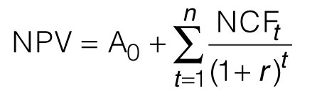
where A0 is the initial cash investment (the cost), which will be negative, r is the discounting rate (also known as the required rate of return) and NCFt is the net cash flow (the benefits accrued) during period t.
(Note: for the non-mathematical, Σ means ‘sum’, the t = 1 subscript says ‘start from the first item’ and the n superscript means ‘continue until all are calculated and summed’.)
Consequently, the minimum criterion for investment in a project proposal is that the net present value is greater than or equal to zero at a given discounting rate.
Recall the proposal with an initial investment of £100 000 that we used to illustrate the payback method. We will use the net cash flow (NCF) for each year to calculate the net present value using a discount rate of 10%. We will not modify the cash flow in year 0 since it represents the present-day value of that cash flow. For each of the subsequent years, we will apply the discounting principle to calculate the present value.
| Year | Net cash flow, NCF (£) | Discounting factor | NPV (£)NPV (£) |
|---|---|---|---|
| 0 | (100 000) | none | (100 000) |
| 1 | 45 000 | /1.1 | 40 909 |
| 2 | 35 000 | 28 926 | |
| /1.12 | (= | 1.21) | |
| 3 | 20 000 | 15 026 | |
| /1.13 | (= | 1.331) | |
| 4 | 20 000 | 13 660 | |
| /1.14 | (= | 1.4641) | |
| 5 | 15 000 | 9 314 | |
| /1.15 | (= | 1.61051) | |
| Total net present value of the proposal’s NCFs = | 7 835 | ||
This result means that, after allowing for financing costs at 10% per annum compounded over 5 years, this proposal will more than pay for the initial investment. In other words, the project is forecast to generate a return that is in excess of 10%. It is financially viable, according to the net present value method. If the NPV were negative, this would infer a return of under 10%.
When two or more proposals of a similar size are being evaluated, the one with the highest NPV will probably be selected. If, at the end of the calculations, a proposal has a negative NPV, it means that the rate of return generated by that proposal is less than the rate required. Unless there were some overriding non-financial reasons for doing so, that proposal would not be implemented.
The chances of reaching the minimum criterion for NPV are affected by the value given to the discount rate. For instance, companies tend to use a discount rate closer to the interest rate for a bank loan rather than the rate associated with a savings account. Some will choose a higher rate to avoid undesired consequences. Many companies use different discount rates depending on the level of risk. High-technology companies may use discount rates of up to 40%. To overcome the difficulty of selecting an appropriate discount rate, it is recommended that you should determine the rate of return implied by the cash flow estimates in a proposal. The result will help management decide whether or not the rate is adequate for their purposes.
SAQ 8
Assume that by investing £20 000 cash in the stock market you could be certain of a 12% rate of return. Now calculate the NPV of proposal B in SAQ 6, using 12% as the discount rate.
Answer
The answer appears in Table S.3.
| Year | Net cash flow £ | Discount factor | NPV £ |
|---|---|---|---|
| 0 | –20 000 | 1.0000 | –20 000 |
| 1 | –2 000 | 0.8929 | –1 785 |
| 2 | 2 675 | 0.7972 | 2 132 |
| 3 | 3 200 | 0.7118 | 2 277 |
| 4 | 4 550 | 0.6355 | 2 891 |
| 5 | 6 550 | 0.5674 | 3 716 |
| 6 | 7 000 | 0.5066 | 3 546 |
| 7 | 8 000 | 0.4523 | 3 618 |
Total net present value of proposal: –£3605.
Internal rate of return (IRR) method
large projects. A small project might have only a modest NPV compared with a much bigger project, but require a much smaller initial investment. To make a ranking possible for projects of different sizes the NPV method may be extended to give a figure called the internal rate of return.
The IRR method calculates the rate of return to be obtained from a proposal, assuming that the discounted values of future cash flows will pay exactly for the initial investment. That is to say, you should look for a discount rate that gives an NPV of zero. The answer is typically found by:
- trying out different rates (typically, by using progressively higher rates) until you find the one that gives you an NPV that is closest to zero
- constructing a graph of NPV for different discount rates until you are confident about the point of intersection of the discount rate axis when the NPV = 0.
Using the same NCFs as the proposal (costing £100 000) we used to illustrate the NPV method, we can try out an increasing series of discount rates as shown in Table 8:
| Rate | Sum | NPV | ||||||
|---|---|---|---|---|---|---|---|---|
| % | Year | 1 | 2 | 3 | 4 | 5 | ||
| NCF (£) | 45 000 | 35 000 | 20 000 | 20 000 | 15 000 | |||
| 10 | 40 909 | 28 926 | 15 026 | 13 660 | 9 314 | 107 835 | 7 835 | |
| 11 | 40 541 | 28 407 | 14 624 | 13 175 | 8 902 | 105 648 | 5 648 | |
| 12 | 40 179 | 27 902 | 14 236 | 12 710 | 8 511 | 103 538 | 3 538 | |
| 13 | 39 823 | 27 410 | 13 861 | 12 266 | 8 141 | 101 502 | 1 502 | |
| 14 | 39 474 | 26 931 | 13 499 | 11 842 | 7 791 | 99 537 | –463 |
Hence, the suggested IRR to get closest to an NPV of zero is 14%. This means that the proposal is worth implementing if management will accept a rate of return of less than 14% per annum (which they would probably do if it were possible to finance the project with a loan with a positive NPV at 12%, say).
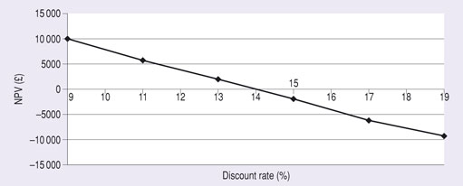
Figure 8 shows a graphical method for finding an IRR for the same proposal using six calculations with different discount rates. It shows an NPV of zero for a discount rate slightly less than 14%. Note that the graph of NPV against discount rate is a curve and not a straight line. While two points, one for an NPV above 0 and one for an NPV below 0, would be sufficient to find an IRR, the level of accuracy is improved by using more data points. If you are using a spreadsheet to find an IRR, the calculations can be used to generate a simple graph like the one shown in Figure 8.
The IRR method is not the only method to use, because it is not always possible to judge the relative viability of proposals by ranking their IRRs. It is preferable to rank similar proposals by their NPVs using the same rate of interest, which is possible when management policy determines the discount rate to use. However, this may not be possible for every financial evaluation. For example, management may not take into account the relative stability of banking interest rates and inflation, as well as their potential fluctuation over time.
SAQ 9
What is the IRR of proposal B (from SAQ 6) to the nearest percentage point?
Answer
A trial and error method is required to establish the value of the discount rate that gives a value of NPV equal to zero. We have already tried 12% and found a large negative NPV so next we might try 6%. You would find that this gave a positive NPV. Successive trials between these values show that at 7% the NPV is still positive (£867), and at 8% it is negative (–£137). You should therefore conclude that the internal rate of return of this proposal is just under 8%.
SAQ 10
To see the effect of project size on the value of IRR and NPV, answer the following questions:
(a) What is the value of IRR of a project twice the size of proposal B in every respect (i.e. all cash flows are doubled)?
(b) What is the effect on NPV of doubling the size of a project?
Answer
(a) The value of IRR is independent of project size.
(b) The value of NPV would be doubled.