

5 End-of-course exercises
This section contains two end-of-course exercises. They are designed to allow you to practise what you have learned in the course and help you to strengthen your understanding of the practical application of the concepts. Since accounting is an applied discipline this is an important step in your learning. The best approach is to attempt the questions by referring to the material in the course if you need to, but without looking at the answers until you have finished.
Exercise 1 Customer profitability
(This question is adapted from Bhimani et al., 2008, pp. 399–400)
Maltloaf produces a soft drink which it distributes to a range of retailers. In addition to the costs of producing the product, Maltloaf has identified a number of customer-related costs, as shown below.
| Activity | Cost driver and rate |
|---|---|
| Order taking | £200 per purchase order |
| Sales visits | £160 per visit |
| Delivery | £4 per delivery mile travelled |
| Product handling | £0.004 per bottle sold |
Maltloaf has collected the following data to facilitate a customer profitability analysis for its four largest customers.
| Smith | Jones | Greene | Browne | |
|---|---|---|---|---|
| Bottles sold | 2,000,000 | 1,600,000 | 140,000 | 120,000 |
| List price | £1.20 | £1.20 | £1.20 | £1.20 |
| Actual price paid | £1.12 | £1.18 | £1.10 | £1.20 |
| Number of purchase orders | 60 | 50 | 30 | 20 |
| Number of sales visits | 12 | 10 | 8 | 6 |
| Number of deliveries | 120 | 60 | 40 | 30 |
| Miles travelled per delivery | 10 | 24 | 40 | 12 |
| Production cost of sales (@ £1 per bottle) | £2,000,000 | £1,600,000 | £140,000 | £120,000 |
Required:
Calculate the operating profit for each customer. Comment on your results, and say which customer(s) Maltloaf would find most attractive.
Discussion
| Smith | Jones | Greene | Browne | |
|---|---|---|---|---|
| Sales revenue (£) | 2,240,000 | 1,888,000 | 154,000 | 144,000 |
| Production cost of sales | 2,000,000 | 1,600,000 | 140,000 | 120,000 |
| Gross profit | 240,000 | 288,000 | 14,000 | 24,000 |
| Gross profit (% of sales value) | 10.71% | 15.25% | 9.09% | 16.67% |
| Order taking | 12,000 | 10,000 | 6,000 | 4,000 |
| Sales visits | 1,920 | 1,600 | 1,280 | 960 |
| Delivery | 4,800 | 5,760 | 6,400 | 1,440 |
| Product handling | 8,000 | 6,400 | 560 | 480 |
| Total customer costs | 26,720 | 23,760 | 14,240 | 6,880 |
| Customer costs (% of sales value) | 1.19% | 1.26% | 9.25% | 4.78% |
| Net profit | Total 213,280 | Total 264,240 | Total (240) | Total 17,120 |
| Net profit (% of sales value) | 9.52% | 14.00% | (0.16)% | 11.89% |
The most notable issues highlighted by this analysis are as follows. (Percentages have been calculated in the analysis, as it often provides greater insights to look at something in terms of its relationship to something else rather than in absolute terms alone).
- There is considerable variation in the gross profit as a percentage of sales and this is due to the discounts from the list price the customers are receiving. Smith receives a large discount, but this is understandable as it is the biggest customer. More surprising is that the biggest discount is received by Greene whose sales volume is extremely low in relation to the two biggest customers, Smith and Jones. Clearly, this is something that Maltloaf’s management should look at.
- Another significant issue revealed is the difference in customer costs in relation to sales revenue, which together with the discounts offered, have a major impact on the operating profit. Most noticeable is Greene, whose customer costs (as a percentage of sales) vastly exceed those of the other customers. The primary cause of this seems to be the disproportionate costs of order taking and delivery. Greene appears to place a relatively large number of purchase orders (i.e. it orders lots of small quantities) and also receives lots of deliveries of relatively small amounts. Compared with the most profitable customer, Jones, Greene’s average order is for 4,667 bottles as against Jones’s 32,000. A similar picture emerges with deliveries: the average number of bottles per delivery for Greene is 3,500 whereas for Jones it is 26,667 (made worse by the fact that Greene also has the longest delivery distance!)
The analysis reveals (in particular) that Maltloaf should renegotiate its terms of trading with Greene, with particular reference to the generous discount offered and the order/delivery batch size. In order to be profitable, and assuming sales volume cannot be increased, Greene would need to buy the same number of bottles in larger orders and with fewer deliveries. It would also need to pay the full list price, as the other small customer, Browne, does.
Exercise 2 Risk, uncertainty and sensitivity analysis
Adapted from: The Association of Chartered Certified Accountants, Paper F9 Financial Management Practice & Revision Kit for exams in 2012. December 2004, Question 27.
Umunat Co (FMC, 12/04)
Umunat Co is considering investing $50,000 in a new machine with an expected life of five years. The machine will have no scrap value at the end of five years. It is expected that 20,000 units will be sold each year at the selling price of $3.00 per unit. Variable production costs are expected to be $1.65 per unit, while incremental fixed costs, mainly the wages of a maintenance engineer, are expected to be $10,000 per year. Umunat Co uses a discount rate of 12% for investment appraisal purposes and expects investment projects to recover their initial investment within two years.
Required:
- a.Explain why risk and uncertainty should be considered in the investment appraisal process.
- b.Calculate and comment on the payback period of the project.
- c.Evaluate the sensitivity of the project’s net present value to a change in the following project variables, then discuss the use of sensitivity analysis as a way of evaluating project risk:
- i.Sale volume
- ii.Sales price
- iii.Variable cost.
- d.Upon further investigation it is found that there is a significant chance that the expected sales volume of 20,000 units per year will not be achieved. The sales manager of Umunat Co suggests that sales volumes could depend on expected economic states that could be assigned the following probabilities:
| Economic state | Poor | Normal | Good |
|---|---|---|---|
| Probability | 0.3 | 0.6 | 0.1 |
| Annual sales volume (units) | 17,500 | 20,000 | 22,500 |
- Calculate and comment on the expected net present value of the project.
Discussion
a.A risky situation is one where we can say that there is a 60% probability that returns from a project will be in excess of $100,000 but a 40% probability that returns will be less than $100,000. If, however, no information can be provided on the returns from the project, we are faced with an uncertain situation. Managers need to exercise caution when assessing future cash flows to ensure that they make appropriate decisions. If a project is too risky, it might need to be rejected, depending upon the prevailing attitude risk.
In general, risky projects are those whose future cash flows, and hence the project returns, are likely to be variable. The greater the variability is, the greater the risk. As the cash flows in capital investment decisions might be for several years ahead, therefore there is bound to be risk involved in such decisions. Therefore, it is highly likely that the actual costs and revenues may either be below or above budget as the work progresses.
- b.Assuming that cash flows occur evenly throughout the year:
Payback =
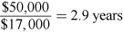
Payback shows how long it will take to recover the initial investment. In this case, the payback period exceeds the company’s hurdle payback period of two years. Therefore, Umunat might be tempted to reject this project. However, a project should not be evaluated on the basis of payback alone. If a project gets through the payback test, it should then be evaluated with a more sophisticated investment appraisal technique, such as NPV. Payback ignores the timing of cash flows within the payback period, the cash flows after the end of payback period and therefore the total project return. It also ignores the time value of money.
| Year | Investment | Contribution | Fixed costs | Net | Discount factor | Total |
|---|---|---|---|---|---|---|
| $ | $ | $ | $ | 12% | ||
| 0 | (50,000) | (50,000) | 1.000 | (50,000) | ||
| 1–5 | 27,000 | (10,000) | 17,000 | 3.605 | Total 61,285 | |
| Total 11,285 |
c.
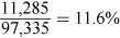
- i.Sensitivity to sales volume
For an NPV of zero, contribution has to decrease by $11,285.
This represents a reduction in sales of
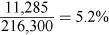
- ii.Sensitivity to sales price
As before, for an NPV of zero, contribution has to decrease by $11,285.
This represents a reduction in selling price of
- iii.Sensitivity to variable cost
As before, for an NPV of zero, contribution has to decrease by $11,285.
This represents an increase in variable costs of

The basic approach of sensitivity analysis is to calculate the project’s NPV under alternative assumptions to determine how sensitive it is to changing conditions. Therefore, sensitivity analysis provides an indication of why a project might fail. Management should review critical variables to assess whether or not there is a strong possibility of events occurring which will lead to a negative NPV. Management should also pay particular attention to controlling those variables to which the NPV is particularly sensitive, once the decision has been taken to accept the investment.
- i.Sensitivity to sales volume
- d.
| Year | Investment | Contribution | Fixed costs | Net | Discount factor | Total |
|---|---|---|---|---|---|---|
| $ | $ | $ | $ | 12% | $ | |
| 0 | (50,000) | (50,000) | 1.000 | (50,000) | ||
| 1-5 | 26,325 | (10,000) | 16,325 | 3.605 | Total 58,852 | |
| Total 8,852 |
The expected net present value is positive, but it represents a value that would never actually be achieved, as it is an amalgamation of various probabilities. Examining each possibility:
| Year | Investment | Contribution | Fixed costs | Net | Discount factor | Total |
|---|---|---|---|---|---|---|
| $ | $ | $ | $ | 12% | $ | |
| 0 | (50,000) | (50,000) | 1.000 | (50,000) | ||
| 1-5 | 23,625 | (10,000) | 13,625 | 3.605 | Total 49,118 | |
| Total (882) |
We already know the NPV of sales of 20,000 units to be $11,285
| Year | Investment | Contribution | Fixed costs | Net | Discount factor | Total |
|---|---|---|---|---|---|---|
| $ | $ | $ | $ | 12% | $ | |
| 0 | (50,000) | (50,000) | 1.000 | (50,000) | ||
| 1-5 | 30,375 | (10,000) | 20,375 | 3.605 | Total 73,452 | |
| Total 23,452 |
The managers of Umunat will need to satisfy themselves as to the accuracy of this latest information, but the fact that there is a 30% chance that the project will produce a negative NPV could be considered too high a risk. It can be argued that assigning probabilities to expected economic states or sales volumes gives the managers information to make better investment decisions. The difficulty with this approach is that probability estimates of project variables can carry a high degree of uncertainty and subjectivity.