2.3.1 Linear magnetic anomalies - a record of tectonic movement

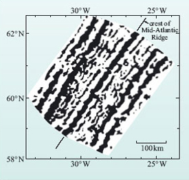
At the time that sea-floor spreading was proposed, it was also known from palaeomagnetic studies of volcanic rocks erupted on land that the Earth's magnetic polarity has reversed numerous times in the geological past. During such magnetic reversals, the positions of the north and south magnetic poles exchange places. In the late 1950s, a series of oceanographic expeditions was commissioned to map the magnetic character of the ocean floor, with the expectation that the ocean floors would display largely uniform magnetic properties. Surprisingly, results showed that the basaltic sea floor has a striped magnetic pattern, and that the stripes run essentially parallel to the mid-ocean ridges (Figure 6). Moreover, the stripes on one side of a mid-ocean ridge are symmetrically matched to others of similar width and polarity on the opposite side.

Figure 6 A modern map of symmetrical magnetic anomalies about the Atlantic Ridge (the Reykjanes Ridge), south of Iceland. (Adapted from Hiertzler et al., 1966)

In 1963, two British geoscientists, Vine and Matthews (Box 1), proposed a hypothesis that elegantly explained how these magnetic reversal stripes formed by linking them to the new idea of sea-floor spreading. They suggested that as new oceanic crust forms by the solidification of basalt magma, it acquires a magnetisation in the same orientation as the prevailing global magnetic field. As sea-floor spreading continues, new oceanic crust is generated along the ridge axis. If the polarity of the magnetic field then reverses, any newly erupted basalt becomes magnetised in the opposite direction to that of the earlier crust and so records the opposite polarity. Since sea-floor spreading is a continuous process on a geological timescale, the process preserves rocks of alternating polarity across the ocean floor (Figure 7a). Reading outwards in one direction from the mid-ocean ridge gives a record of reversals over time, and this can be matched with the record read in the opposite direction.

Figure 7 (interactive): The animation in Figure 7 below shows the pattern of magnetic reversals on either side of a mid-ocean ridge. Black = normal magnetic field; white = reversed field. When these reversal data are combined with age data (derived by radiometric dating of rocks dredged from the sea floor), a geomagnetic timescale can be produced, as you can see in the right of the animation. Detailed geomagnetic timescales have now been produced for all of the geological time since the Jurassic Period.

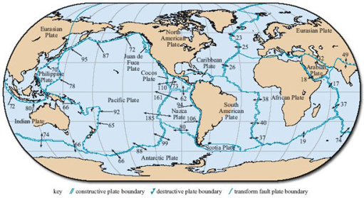
Magnetic and oceanographic surveys of the ocean floor have collected information on both its palaeomagnetic polarity and its absolute age (by radiometric dating of retrieved sea-floor samples). Combining these two records has helped establish a geomagnetic timescale (Figure 7b) and, by using samples from the oldest sea floor, this timescale has now been extended back into the Jurassic Period, allowing the ages and rates of sea-floor spreading to be established for all the world's oceans, as shown in Figure 8. (The different types of plate boundary shown in Figure 8 are discussed later in the text.)

Maximise

Figure 8 Map showing the global distribution of tectonic plates and plate boundaries. The black arrows and numbers give the direction and speed of relative motion between plates. Speed of motion is given in mm y⁻¹. (Adapted from Bott, 1982)

Click on 'View document' below to see a larger version of the above image.

Two measures of spreading rate are commonly cited:

• where the rate of spreading is determined on one side (i.e. the rate of movement away from the ridge axis), this is termed the half spreading rate;

• where the rate is determined on both sides (i.e. the combined rate of divergence), the combined value is termed the full spreading rate.

Activity 3

The width of ocean floor between the spreading ridge in the South Atlantic Ocean at 30°S and the edge of the continental shelves along the east coast of South America and the west coast of southern Africa at 3°S is approximately 3100 and 2700 km respectively. Assuming that the spreading rate on this segment of the ridge is 38 mm y⁻¹, estimate the maximum age of the sea floor on either side of the South Atlantic.

Answer

For the South Atlantic Ocean:

The age of ocean crust (t) adjacent to the South American continental shelf is derived from:

The age of ocean crust adjacent to the southern African continental shelf

Magnetic stripes not only tell us about the age of the oceans, they can also reveal the timing and location of initial continental break-up. The oldest oceanic crust that borders a continent must have formed after the continent broke apart initially, and just as sea-floor spreading began. In effect, it records the age when that continent separated from its neighbour. In the northern Atlantic, for example, oceanic crust older than 140 Ma is restricted to the eastern USA and western Saharan Africa, therefore separation of North America from this part of Africa must have commenced at this time. The oldest oceanic crust that borders South America and sub-equatorial Africa is only about 120 Ma old. Accordingly, it follows that the North Atlantic Ocean started to form before the South Atlantic Ocean.

If new sea floor is being created at spreading centres, then old sea floor must be being destroyed somewhere else. The oldest sea floor lies adjacent to deep ocean trenches, which are major topographic features that partially surround the Pacific Ocean and are found in the peripheral regions of other major ocean basins. The best known example is the Marianas Trench where the sea floor plunges to more than 11 km depth. Importantly, ocean trenches cut across existing magnetic anomalies, showing that they mark the boundary between lithosphere of differing ages. Once this association had been recognised, the fate of old oceanic crust became clear - it is cycled back into the mantle, thus preserving the constant surface area of the Earth.