4 Your formulas – using a spreadsheet
Although there may be many occasions when you are given a formula to use, sometimes you may need to devise your own formulas, for example if you use a spreadsheet on a computer at home or at work. This section looks at the process of devising a formula in more detail.
Part of a spreadsheet that has been constructed to record monthly income and expenditure is shown below. It is similar to a balance sheet that you might draw up by hand and includes the monthly income and outgoings, the totals and the overall balance. It is used to keep track of expenditure, particularly to try and ensure that the balance remains positive. However the spreadsheet has been stored on a computer rather than on paper and is updated regularly. One of the advantages of using a computer spreadsheet is that you can insert formulas into the spreadsheet to carry out the necessary calculations automatically, without using your calculator.
A spreadsheet is made up of rows and columns of cells. The columns are identified by letters and the rows by numbers. This enables you to identify each cell in the spreadsheet. For example the number 110.56 is in column B, row 11, so this cell is B11.
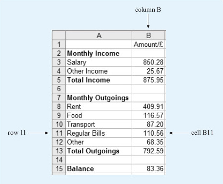
Cells can be found from their reference, by looking down the column and across the row. So cell A3 can be found by looking down column A and across row 3. This cell contains the word ‘Salary’. Notice that cells can contain either text or numbers.
Activity 10: Spreadsheet cells
a.What is contained in the following cells?
i.A5
ii.A12
iii.B15
iv.B1
b.What is the reference for the cells that contain the following?
i.The number 792.59
ii.The word ‘Food’
Discussion
a.
i.The cell that is in both column A and row 5 contains the words ‘Total Income’.
ii.Looking down column A and across row 12, cell A12 contains the word ‘Other’.
iii.The cell that is in column B, row 15 contains the number 83.36.
iv.The cell that is in column B, row 1 contains the heading ‘Amount /£’. This indicates that the entries in this column are amounts of money and that they are measured in £. This heading could also have been written as ‘Amount in £’ or ‘Amount (£)’.
b.
i.792.59 is in column B and row 13, so its reference is B13.
ii.‘Food’ is in column A and row 9, so its reference is A9.
Now have another look at the spreadsheet and see if you can work out what information it shows. For example, if you look at row 3, this shows that the monthly salary is £850.28. Although cell B3 only contains the number 850.28, you know that this is measured in pounds from the heading in cell B1. Overall, the spreadsheet shows the different items that make up the monthly income and where money has been spent over the month as well. If you were keeping these records by hand, you would then need to calculate the total income, the total outgoings and the balance.
For example, to find the total income for the month, you would need to add the salary (£850.28) to the other income (£25.67). This gives the total income of £875.95. In other words, to calculate the value in cell B5, you need to add the values in cells B3 and B4 together. This can be written as the following formula:
value in B5 = value in B3 + value in B4
Activity 11: Finding the balance
Formulas have also been used to calculate the total monthly outgoings and the balance. If you were working these calculations out by hand, what would you do? Check by comparing your answers with the values in cell B13 and B15. Try to write down the formulas for these cells in the form ‘value in B13 = …’.
Discussion
To calculate the total monthly outgoings, you need to add up the individual outgoings on ‘Rent’, ‘Food’, ‘Transport’, ‘Regular Bills’ and ‘Other’. So the formula will be:
value in B13 = value in B8 + value in B9 + value in B10 + value in B11 + value in B12
To find the balance, you need to take the outgoings away from the total income. So the formula will be:
value in B15 = value in B5 − value in B13
To put these formulas in the spreadsheet, you can type the formula directly into the relevant cell, starting with an equals sign to show that you are entering a formula rather than a word.
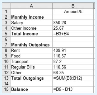
Notice that in cell B13, a shorthand form for the sum has been entered. You could have typed in = B8+B9+B10+B11+B12, but it is also acceptable to use the shorthand form, = SUM(B8:B12), which is shown here. This instruction tells the computer to add together the values in all the cells from B8 to B12.
One of the advantages of using a spreadsheet is that if you change some of the numbers, all the calculations that use that particular number will be automatically updated to reflect the change. For example, in this budget the amounts for the salary, rent and the regular bills are likely to remain the same from one month to the next and may only be updated once or twice a year. However, the amounts for food, transport, other bills and other income probably will change from month to month. These values can be changed easily on the spreadsheet and the revised balance produced immediately.
Activity 12: Spreadsheet formulas
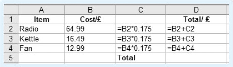
The formulas used in a spreadsheet are shown in the diagram below. Note that * is the notation for multiplication and / is the notation for division.
-
(a) The values in columns C and D are displayed to two decimal places as they represent an amount of money. What values will be displayed in cell C3 and cell D3?
-
(b) What do you think is being calculated in the cells in column C? Can you suggest a suitable heading for this column, to be entered into C1?
-
(c) Cell D5 should contain the total of the values in D2, D3 and D4. Write down a formula that could be entered in cell D5. What does this value represent?
Discussion
-
(a) The formula in C3 is:
-
value in C3 = value in B3 × 0.175.
-
So the value in C3 = 16.49 × 0.175 = 2.885 75.
-
Although the full value is kept in the cell, it will only be displayed to 2 d.p. as 2.89.
-
The value in D3 is obtained by adding together the values in B3 and C3.
-
So, value in D3 = value in B3 + value in C3 = 16.49 + 2.885 75 which is 19.375 75. This will be displayed to 2 d.p. as 19.38.
-
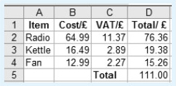
(b) The numbers in column C are 0.175 or 17.5% of the values in column B. You may know that 17.5 % is the main UK VAT rate, so it looks as if column C represents the amount of VAT paid on the different items described in column A. A suitable heading might be VAT/£ or VAT in £ or VAT (£).
-
(c) The total can be found by adding together the values in cells D2, D3 and D4. So the formula ‘= D2+D3+D4’ could be entered into cell D5. Alternatively, you could use ‘=SUM(D2:D4)’. This represents the total cost (including VAT) of the radio, kettle and fan.
With these changes, the spreadsheet will look like the following.