
2.5.1 Physical and weather-related indicators
The indicators collected in Table 4 have been observed to change over large regions of the Earth during the 20th century. According to the TAR, there is now a good level of confidence that what is being recorded is the result of long-term change rather than short-term natural fluctuations. As we noted earlier (Section 2.2.2), the most recent period of warming has been almost global in extent, but particularly marked at high latitudes. So are the changes in Table 4 consistent with rising temperatures on both a regional and global scale?
| Weather indicators | Observed changes* |
|---|---|
| hot days/heat index† | increased (likely) |
| cold/frost days | decreased over most land areas during 20th century (very likely) |
| continental precipitation | increased by 5-10% over 20th century in Northern Hemisphere (very likely), although it has decreased in some regions (e.g. N and W Africa and parts of Mediterranean) |
| heavy precipitation events | increased at mid- and high northern latitudes (likely) |
| frequency and severity of drought | increased summer drying and associated incidence of drought in a few areas (likely); in recent decades, frequency and intensity of droughts have increased in parts of Asia and Africa |
| Physical indicators | Observed changes* |
|---|---|
| global-mean sea level | increased at average annual rate of 1-2 mm during 20th century |
| duration of ice cover on rivers and lakes | in mid- and high latitudes of Northern Hemisphere, decreased by 2 weeks during 20th century (very likely); many lakes now freeze later in autumn and thaw earlier in spring than in 19th century |
| Arctic sea-ice extent and thickness | thinned by 40% in recent decades in late summer (likely), and decreased in extent by 10-15% since 1950s in spring and summer |
| non-polar glaciers | widespread retreat during 20th century |
| snow cover | decreased in area by 10% since satellite observations began in 1960s (very likely) |
| permafrost | thawed, warmed and degraded in parts of polar and sub-polar regions |
* Levels of confidence (Box 8) where available are given in brackets.
† Heat index is a measure of how humidity acts along with high temperature to reduce the body's ability to cool itself.
Question 9
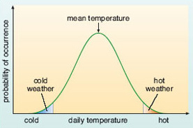
(a) Figure 29 is a schematic representation of the distribution of daily temperatures (for a fictional location), scattered around the mean value according to a bell-shaped curve (a 'normal' distribution). At the tail ends of the distribution, the shaded areas represent the frequency of occurrence of unusually cold (left) and unusually hot (right) days. Suppose now that the mean temperature increases, but the distribution of temperatures around the mean (i.e. the shape of the curve) is unchanged. Sketch a second curve on Figure 29 to represent this 'new' climate, and use it to explain the first two weather-related entries in Table 4.
(b) Drawing on your own experience, how might the shifts you identified in part (a) be expected to affect the human death-toll due to temperature extremes?
Answer
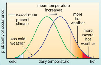
(a) Figure 30 shows how an increase in mean temperature shifts the wholebell-shaped curve to the right. This reduces the frequency of unusually cold days (effectively to zero, in the somewhat exaggerated situation depicted to the left in Figure 30), and increases the frequency of unusually hot days (i.e. the area under the curve above a given temperature, to the right in Figure 30, is now much larger). This pattern is consistent with the first two entries in Table 4.
(b) Shifts of the kind identified in (a) could have both beneficial effects (reducing the number of cold-related deaths in winter in some regions) and adverse effects (increasing the number of deaths due to heat stress).
The remaining weather indicators in Table 4 (changes to precipitation and droughts) are less easy to link directly with a rise in GMST. However, they do bear directly on one of the major reasons for concern about regional climate change - a possible increase in extreme events
SAQ 27
What about the changes in physical systems collected in Table 4? How might these be explained by rising temperatures?
Answer
The thinning and reduced extent of snow and ice cover over land and sea, and the melting of permafrost (Box 9), are all consistent with a warming of the climate. We might also expect that this warming has, in turn, contributed to the observed sea-level rise, both through direct warming and thermal expansion of seawater (Box 4; Section 1.3.4), and because the widespread melting of glaciers has added more water to the oceans.
Sea-level rise is one of the most feared aspects of global warming for island nations like Tuvalu, and for inhabitants of other low-lying parts of the planet. Yet keeping tabs on global mean sea level (the indicator included in Table 4) is, if anything, an even more complicated problem than monitoring the Earth's temperature - and again provides scope for disagreement and controversy among scientists.
Today, sea-levels are recorded by coastal tide gauges relative to a fixed benchmark on land. Averaged over a period of time (a year, say, to remove short-term effects due to waves, tides, weather conditions, etc.), the result is the local 'mean sea level'. The difficulty in interpreting changes in mean sea level at a particular locality is that the land moves up and down as well. These vertical land movements can result from human activities (of the kind noted in connection with Bangladesh in Box 9), or more generally from natural causes - including tectonic processes (e.g. earthquakes) and very slow adjustments to major changes in ice-loading. For instance, the UK is still adjusting to the melting of ice at the end of the last glacial period; Scotland is rising a few mm a year and the south of England is sinking at a similar rate.
With this in mind, you can begin to see why it might be difficult to establish how global mean sea level (sea level averaged across the globe) has varied over the past century due solely to changes in the total volume of water in the oceans. It is this so-called 'eustatic' sea-level change that is linked to the climate-related factors identified above: thermal expansion of seawater and melting of land ice. All the historical records from tide gauges around the world measure only relative sea level. Not only is the spatial distribution of high-quality long-term records decidedly patchy, but individual records must also be adjusted for local land movements. This is a major source of uncertainty in the IPCC estimate included in Table 4.
SAQ 28
What does this estimate imply about the total sea-level rise over the 20th century?
Answer
A rate of increase of 1-2 mm per year translates into a rise of 10-20 cm in the past 100 years.
But is this linked to 20th century climate warming? There is no independent evidence of this. All scientists can do is to estimate the contributions due to the observed warming, and see whether this matches the observed sea-level rise. The IPCC TAR estimates of the various temperature-linked contributions are collected in Table 5. Some background information on these estimates is given in Box 10. Read through that material, and then try Question 10.
| Low | Central estimate | High | |
|---|---|---|---|
| effects due to 20th century warming: | |||
| thermal expansion | 0.3 | 0.5 | 0.7 |
| glaciers | 0.2 | 0.3 | 0.4 |
| Greenland ice sheet | 0.0 | 0.05 | 0.1 |
| Antarctic ice sheet | −0.2 | −0.1 | 0.0 |
| long-term ice-sheet adjustment | 0.0 | 0.25 | 0.5 |
| total estimated | 0.3 | 1.0 | 1.7 |
| observed | 1.0 | 1.5 | 2.0 |
Box 10 Glaciers and ice sheets: how do they respond to climate warming?
The ice stored on land is usually carved up into two broad categories:
Glaciers (and small ice caps) in mountainous areas (such as the Alps, Andes, Himalayas, etc.) and at high latitudes (in places like Iceland, Alaska, the Canadian Arctic and Scandinavia).
The vast ice sheets in Greenland and Antarctica.
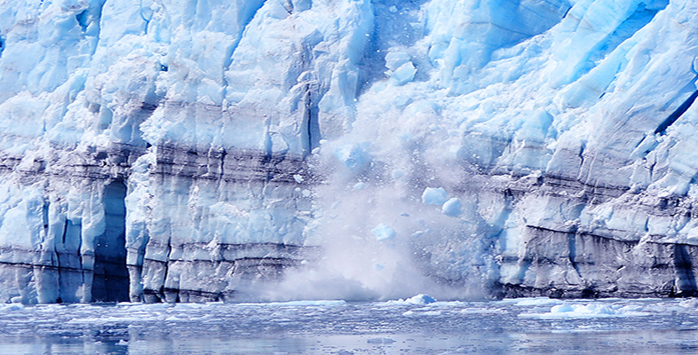
A glacier or ice sheet gains mass by accumulation of snow (which is gradually transformed to ice) and loses mass (known as ablation) mainly by melting at the surface or base, with subsequent runoff or evaporation of the meltwater. Bodies of ice have their own internal dynamics as well. Ice is deformed and flows within them - down a mountain for example, or in vast slow-moving 'ice streams' within the major ice sheets. Where a glacier or ice stream meets the sea, ice may be removed by the calving of icebergs or by discharge into a floating ice shelf (Figure 31), from which it is lost by basal melting and calving of icebergs.
How climate warming affects the total mass of an individual glacier or ice sheet depends on how the balance between accumulation (through snowfall) and ablation (through melting and discharge) responds to rising temperatures. On the face of it, this is a simple task of relating climate to accumulation and loss rates. In practice, numerous factors conspire to complicate this simple picture - not least the internal dynamics of the ice body.
Nevertheless, estimates of glacier and ice-sheet sensitivity to climate change have been made. On the basis of such estimates, a warmer climate is judged to result in a shrinkage of glaciers and the Greenland ice sheet, due to increased ablation. By contrast, Antarctic temperatures are currently so low that modest warming is expected to increase the overall mass of ice, due to increased accumulation accompanying a warmer atmosphere with increased moisture availability.
One final, very important complicating factor: the mass balance of a body of ice is essentially always attempting to catch up with climate. There is a time lag between climate change and the corresponding effect on a glacier or ice sheet, known as the response time.
In general, glaciers are not only pretty sensitive to climate change, they also have relatively short response times - typically 50 years or so, though the actual value varies depending on surface area, ice thickness and other factors. By contrast, changes in ice discharge from ice sheets have response times of 1000 years or more. Hence, it is likely that the Greenland and Antarctic ice sheets are still adjusting to their past history, especially the last glacial/interglacial transition. Table 5 includes an estimate of the contribution this long-term adjustment has made to 20th century sea-level rise.
Question 10
(a) Using the central estimates in Table 5, work out the percentage contribution each factor has made to the mean rate of sea-level rise during the 20th century. Which of these factors appears to have made the major contribution?
(b) In broad terms, are the estimated contributions from glaciers and the major ice sheets (due to 20th century warming) consistent with the background information in Box 10?
Answer
(a) From the central estimates in Table 5, the major contribution to the observed rate of sea-level rise has come from the thermal expansion of seawater; this accounts for (0.5/1.5) × 100% = 33%. The next-largest contribution was due to melting glaciers (20%), followed by 'long-term icesheet adjustment' (17%; this is something that will continue to make a significant contribution in future), and then loss of ice from the Greenland ice sheet due to 20th century warming (just 3%).
(b) The short answer is 'yes'. According to Box 10, glaciers and the Greenland ice sheet are expected to lose mass in a warmer climate (greater ablation exceeds any gains from increased precipitation), but glaciers respond much more quickly. By contrast, the Antarctic ice sheet is expected to gain mass (due to increased precipitation), which is consistent with the negative entry in Table 5 (i.e. this has partly offset the loss of ice elsewhere).
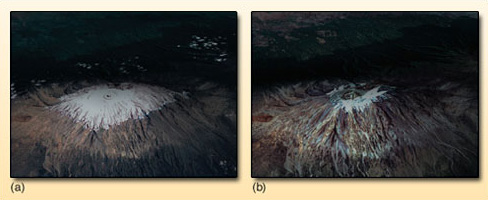
Clearly, there are large uncertainties associated with the estimates collected in Table 5. This reflects a lack of sufficient observational data, inadequate understanding of the complex processes involved and shortcomings in the models used to produce some of these estimates. For instance, there is abundant evidence that the 20th century saw widespread glacier retreat across the globe: from the Arctic to Peru and New Zealand, from Switzerland to the Himalaya (Box 9) and the famed snows of Mount Kilimanjaro (Figure 32), vast ice fields and glaciers are shrinking. Yet it is still a difficult and uncertain business to quantify the loss of ice and assess its impact on the total volume of water in the world's oceans.
Meanwhile, the sheer physical size and inaccessibility of the ice sheets, the extreme climates and the occurrence of long periods of polar darkness have long rendered the acquisition of representative measurements extremely difficult. For example, the lack of suitable long-term data means there is no direct evidence that the whole Greenland ice sheet did actually shrink during the last 100 years; the estimate in Table 5 is based entirely on modelling studies driven by the observed warming over the ice sheet. However, satellite surveillance has been in place since 1990, and this short-term record does indicate a rapid thinning of the edges of the ice sheet.
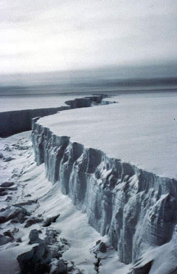
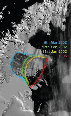
Summaries of available data for the whole of Antarctica have tended to find small positive net mass balances overall (in line with the estimate in Table 5), though with high degrees of uncertainty. But once again, there are signs that dramatic change is underway in some parts of the continent - not least the recent rapid collapse of several ice shelves around the Antarctic peninsula (Figure 33). Despite the newspaper headlines that accompany such an event, bear in mind that disintegration of a floating ice shelf does not, by itself, contribute to sea-level rise. (If you want to prove this for yourself, try floating ice cubes in a tumbler brimful of water to see if it overflows as they melt.) However, there is concern that, without ice shelves to act as dams, the continent's ice streams and glaciers might migrate faster towards the coast, ultimately contributing to sea-level rise. There are early indications that this may be happening in some parts of western Antarctica.
SAQ 29
Now have another look at the estimates in Table 5. Taken together, do they tell the whole story of sea-level rise during the 20th century?
Answer
Probably not. The uncertainties are large, but (based on the central estimates) these climate-related contributions make up only some 67% of the observed rate of increase. However, the high estimate does account for the observed rise.
The IPCC identified the influence of some additional factors (not directly related to climate change, such as the extraction of groundwater), but were still left with a discrepancy between the estimated and observed rate of sea-level rise. Given the uncertainties that pervade this issue on all fronts, this is not altogether surprising. Nevertheless, the TAR concluded that 'it is very likely [90-99% probability; Box 8] that the 20th century warming has contributed significantly to the observed sea-level rise'.