6 A problem with sensors

The problem we will look at in this section concerns the analysis of the design of a component used in cars that are fitted with airbags. The airbag has to be inflated rapidly when an electronic circuit in the system decides that a serious collision is taking place. The crucial component in the electronics is the accelerometer, which therefore has to be extremely reliable. Motor manufacturers have turned to a technology called MEMS (micro-electromechanical systems) for these accelerometers, because it enables large numbers of devices to be made at low cost, but with fantastically high reliability. The sensors are made on silicon chips, using the same manufacturing methods and equipment as electronic chips, the difference being that the results are mechanical structures rather than transistor circuits. Figure 32 shows an example of such a sensor. Notice the scale of the device.

Figure 32 Detail of a typical MEMS accelerometer

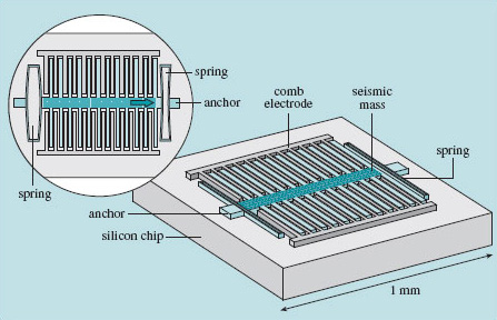
Most airbag accelerometers are of the type shown in Figure 32. They consist of a silicon chip, into which the sensor and the sensing structure are fashioned. It is made entirely of silicon and is in two parts: the first is a lump (often called the proof mass or seismic mass) suspended by means of a spring formed at each end; and the second is a pair of fixed sensing electrodes that enable the electronics to detect the movement of the lump relative to the surrounding platform of silicon.

The way it works is like this: when the chip is subjected to an acceleration, the lump moves a little relative to the chip and the fixed structures on it, in the same way as your shopping might fall off the back seat of the car if you brake hard. The amount of movement depends on the size of the acceleration, the stiffness of the springs, and the mass of the lump. When the lump is deflected, the electrical capacitance between it and the sensing structures on the chip changes, and this change is detected by the electronics, which converts it to a value for acceleration.

From the point of view of building prototypes and mock-up devices to test and refine the design, the trouble with MEMS is that the things you make are very small – too small to poke with a finger to see how they're working, and too small to measure directly how much they move when the acceleration is applied. You can't even build a scale model and make the measurements on that instead, because the material properties don't all scale up in the same way. Crucially for the accelerometer, the mass is proportional to the length-scale cubed (because mass is directly related to volume, not length), but the stiffness of the support springs would scale only in proportion to their length. Therefore, you would have to build your scale model out of a different material from the silicon of the real device if you wanted to mimic its behaviour on a magnified scale whilst maintaining the same ratio of mass to stiffness. A material with the right combination of properties probably doesn't exist.

You can go some of the way towards being sure that your design will work just by doing hand calculations. For instance, you would be able to calculate the stiffness of the springy support structure by using the appropriate formula for a beam of that type. This would enable you to estimate how far the mass would move under a given acceleration. Things get much more difficult if you want to predict how much it will bend if subjected to a sideways acceleration, because the manufacturing process demands that it has lots of holes in it. This makes the structure very complicated, and the standard equations for stiffness of uniform beams don't apply.

So, to test different designs of accelerometer, it looks as though you may have no choice but to make some for real. Unfortunately, the set-up costs for small runs of MEMS devices is very high (electronic chips are cheap only because millions of them are made at the same time).

The way out of this is to use finite element analysis (FEA) to check as many aspects of the device's behaviour as possible before spending money on building any.

FEA is most commonly used to find out what happens to a structure when a mechanical load is applied to it, but it has many more applications. It can be used to predict the temperature distribution in a central heating boiler, the blood flow patterns around an artificial heart valve, the acoustics of a loudspeaker, or the magnetic fields in an electric motor. In short, anything where there is an interaction between a field (e.g. temperature, magnetic, electrostatic, acoustic, flow, force) and an object.

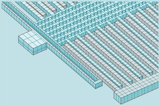
FEA solves the difficult differential equations that are involved by breaking the problem up into many smaller, but related problems. A computer is used to solve a huge number of Box 11 Simultaneous equations , and the solution to the whole problem is presented as a visual display in two or three dimensions. Figure 33 shows a computer model of the accelerometer, ready for analysis by the FEA program.

Figure 33 Seismic mass of MEMS accelerometer, showing meshing

Box 11 Simultaneous equations

I'm going to present a simple example of simultaneous equations, to illustrate why they crop up in FEA, and why we need computers to solve them even though the equations themselves may be quite straightforward. First, to remind you about simultaneous equations: they occur whenever you want to find the answer to a question where more than one condition has to be satisfied at the same time.

Cutting a piece of wood

A trivial example will get us started. Suppose you have a piece of wood 2.4 m long that you want to cut into two, with one piece four times the length of the other. This problem is so simple that you would do it in your head without realising that you had been solving simultaneous equations, but bear with me as I go in slow motion through the process, as it illustrates the general principle.

The two conditions that must be satisfied give rise to the two simultaneous equations that describe this problem. In ordinary language they are:

'The length of both pieces added together equals 2.4 m.'

'The length of one piece equals four times the length of the other piece.'

If you call the length of one piece x, and that of the other y, then:

By substituting the second equation for x into the first, we can rewrite the first equation like this:

and we quickly find that

Now that we know y, we can use either of our original equations to find that

Our results for x and y are in metres, of course.

A system of springs

We need to take this example a step further to give an insight into why we get simultaneous equations in FEA. If you reformulated the woodcutting problem in terms of springs and forces, you could say: 'I have two springs, but one is four times as stiff as the other. They are linked end to end, and the pair is anchored at one end (Figure 34). I move the free end by a distance of 2.4 mm; how far has the point where the two springs are linked moved?

Figure 34 Linked spring system, showing extension

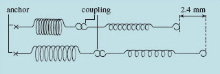
The force that has been applied to move the free end of the pair of springs is transmitted throughout the spring system, so we know that the force acting on each spring is the same. In a spring, the amount it extends and the force pulling it are related by the stiffness, through the expression F = kx, where F is the applied force, k is the stiffness, and x the extension.

We have said that the stiffness k ₂ of one spring is four times that of the other, k ₁. We can write this as:

We have just said that the force experienced by each spring is the same, so we can also say that

where x is the extension of one spring, and y that of the other. We can get rid of the k terms by saying

and so

This is the first of our simultaneous equations, and it says 'the amount the first spring stretches is four times as much as the second spring'.

The other equation states that the extension of both springs added together is 2.4 mm.

So,

We needn't go through the maths because it is exactly the same as the wood-cutting example (except that our results will be in millimetres).

The point between the two springs and the end where the force is applied are effectively nodes in a simple finite element mesh. The springs are just representations of the stiffness of the material. What we have just solved is a small finite element problem. In a real problem, the numbers of calculations that need to be made are much bigger, and we may have 10 000 nodes and 30 000 simultaneous equations, which is why we use a computer. The calculations are generally rather more complex than in the spring example, because usually we are dealing with continuous materials, not 'lumps' like the springs, and there may also be non-linear behaviour.

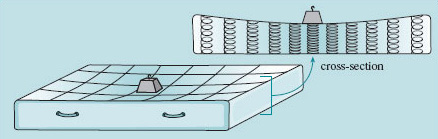
If instead of two springs we had ten, each with a different stiffness, we could fairly comfortably still solve this by hand, to get the new positions of each node. But what if the springs extended in two or three dimensions, as in Figure 35?

Figure 35 2-D and 3-D arrays of linked springs

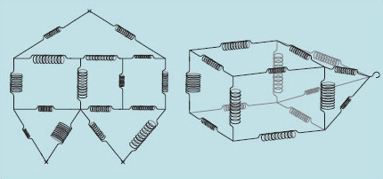
The array of springs now resembles a mattress (Figure 36). Imagine a weight were placed on it. You can see how this would now be very awkward to calculate, because the depression of the mattress would cause some of the springs representing the upper and lower fabric skins to change the direction in which they pull, according to how close they are to the weight. The awkwardness comes in the large number of interdependent calculations (simultaneous equations) and that is where a formal approach and the power of a computer are able to come to the rescue.

Figure 36 Cross-section of a mattress with a weight on it

Returning to finite element analysis, the structure (in the case of the accelerometer, the mass and springs) is first divided up into a large number of small blocks, or elements. The size and shape of these elements can vary. They are made to be much smaller than any features of the structure near them. Usually, their form is tetrahedral or hexahedral (i.e. with four or six faces), but the essential properties they have are that they completely fill the volume of the structure, and that they are connected to their neighbours at their vertices. These elements are usually not regular shapes – they have to be distorted to fit the geometry of the structure being analysed, which could have any shape. Within reason, this distortion does not matter, provided that the elements are properly connected to their neighbours.

If enough elements are used, the continuously varying quantity that is to be determined (in our case the displacement) can be approximated into simpler variations within each element (for example, a linearly varying displacement across the element). According to their position in the structure, each element is assigned material properties. These properties are used to solve, for each element, what is happening within it. Because each node of each element is shared with neighbouring elements, the whole assembly of elements is linked, and the solution arrived at for each element is consistent with those arrived at for all its neighbouring elements.

The process of dividing the structure into these discrete elements is called meshing. The size of the elements in a mesh needs to be considered carefully: if the elements are too large relative to the structure, the result of the analysis will be inaccurate; if they are too small, the analysis may take far too long for the computer to execute. In modern FEA software packages, much of the routine and arduous work of meshing has been taken away, so that the meshes are generated automatically by the software, once the user has answered some questions such as what type of element they want to use.

But all we have done so far is divide the structure into elements and told the computer what they are made of. The program needs to be set going somehow, and this stage is known to FEA practitioners as 'setting the boundary conditions'. The computer needs to be told what other things are known about the problem. This is in a quite literal sense setting out what is happening at the boundaries or edges of the structure. In the case of the accelerometer, you would apply a direction and magnitude for an acceleration. Another boundary condition would be where the mass is attached to the silicon chip, and what sort of attachment this is. Is it fixed in position but free to rotate about one or more axes, or can it slide in one direction?

The deflection of a material, and the stress generated due to an applied load, are simply related to one another by the stiffness of the material. Therefore, solving the problem for deflection also provides the solution for stress. Figure 37 shows the results of running a finite element analysis of a MEMS accelerometer seismic mass subjected to a sideways acceleration. The colour shading shows where the stresses are concentrated.

Figure 37 FEA results showing stress distribution on MEMS accelerometer

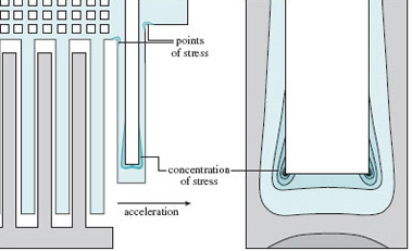
One important thing to understand about FEA is that there are many opportunities to create a result that looks convincing, but is completely incorrect. Meshing is one such opportunity – usually where the mesh is too coarse to allow accurate calculation. This is most likely to happen near features in the structure, such as holes and corners, as in Figure 38. This is why in a properly meshed structure the element size is smaller around such features than elsewhere.

Figure 38 FEA results for stresses around a circular hole in a square plate, using different mesh sizes. Notice the difference in the results: (a) is inadequately meshed

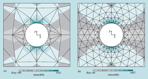
It is good practice when doing FEA to run what is called a meshing analysis. This is where the same structure and boundary conditions are run with three or four different levels of mesh refinement, and the results are compared with one another. You can have reasonable faith in the quality of a mesh when the answers are very similar for two different levels of refinement of the mesh. But it is possible to go too far: if the elements get so small as to approach the size of the microstructure of the material (e.g. grains in a metal), then the implicit assumption in FE modelling – that the material is continuous – breaks down.

Another common source of error is incorrectly specified boundary conditions; for example, the wrong type of constraint at anchor points. In the accelerometer, the anchor points are where the springs are attached to the substrate. These should be defined as constraining motion in all three translations and all three rotations.

All this points to a need for independent verification of the results, and this often involves doing real tests on real structures. Ordinary hand calculation is useful too, because even if it doesn't give you accurate data, it is normally possible to get an estimate within a factor of two or three of the right answer, and this allows you to spot really gross errors in the FEA results. The FEA software companies also provide large numbers of worked examples of standard problems to allow you to check that your model behaves correctly.

To sum up these thoughts on the shortcomings of FE analysis, we can say that what we are working with is only a model, and models by their nature are never exactly like the real thing. The skill of the engineer lies in knowing how far the model can be stretched and how deeply probed, and yet still yield information about the real world.