

2.6 Pressure variations in one place
So far, when we have been thinking about pressure waves we have visualised a pattern of pressure variations extending through space, and travelling away from the source of the vibration.
I now want to consider how the pressure variations change at one particular place in the vicinity of the tuning fork as time passes. You could think of this as examining how the pressure at your eardrum varies from moment to moment as you listen to a tuning fork's sound, or how the pressure changes at any fixed point in the vicinity of a source or instrument.
We can consider the progress of a wave with respect to time by looking at a pressure wave reaching a detector at a fixed point. At one instant in time a region of high pressure is detected with the arrival of a compression, at the next the detector might detect normal pressure followed then by low pressure. These variations in pressure will occur at regular periodic time intervals, and the plot of pressure versus time would appear as a sine curve with the crests of the wave again corresponding to compressions and the troughs to low pressure regions. In this case the measurement in time from one compression to the next is given by the period of the wave – the time taken for one cycle. The reciprocal of this, that is one over the period, is called the frequency. It is equivalent to the number of cycles per second and has the unit ‘hertz’. We shall be looking at frequency in more detail shortly.
Figure 10(b) shows a graph with a familiar sinusoidal shape.
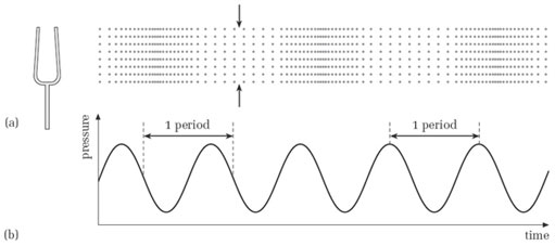
It is important to appreciate the distinction between the graph in Figure 10(b) and the one shown earlier in Figure 6(b). In Figure 6(b), it was as though we could survey the whole of the region in which the tuning fork was audible, and at a particular instant see where the high-pressure regions were and where the low-pressure regions were. In Figure 10 we are focusing our attention on one region of space, such as that between the pair of arrows in Figure 10(a), and observing what happens as time passes rather than at one instant of time. The graph in Figure 10(b) shows the variations of pressure in this region as the wave goes by. It has the familiar sinusoidal shape, but the pressure is shown as a variation with time instead of with distance. (Notice that the horizontal axis now carries the label ‘time’.)
Just as the prongs of the fork cyclically go backwards and forwards, so the pressure at any particular point, such as that indicated by the arrows, cyclically rises and falls. In other words, the pressure variations at any point are periodic, just as the motion of the fork's prongs are periodic. In the time it takes for the prongs to complete one cycle of movement there is one complete cycle of pressure variation (from high to low and back to high again, for instance). Hence, the period of one complete cycle of pressure variation is the same as the period of the tuning fork.
The duration of a cycle (the period) is the time interval between any two corresponding points on consecutive cycles of the pressure wave. Figure 10(b) shows the period marked at two different places on the graph, but there are infinitely many places from which to measure the period of the oscillation.
Activity 11 (Self-Assessment)
What are the periods of the pressure variations represented by the graphs in Figure 11?
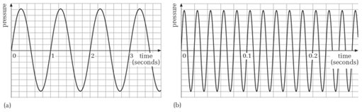
The period of the waves encountered in music is generally very short. For instance, a typical value might be 0.001 s, or a thousandth of a second. When dealing with such short times as these, it is often more convenient to use the millisecond as the unit of time. One millisecond (1 ms) is a thousandth of a second (or 1 × 10⁻³ s).