

2.3 Other influences on market demand
What about other variables which may affect demand? Let us consider four such variables. As is often the case in economics, the first two points involve understanding some rather formal relationships between variables, in this case price and income.
The price of other goods. Two goods x and y are known as substitutes if the quantity demanded of good x increases after a rise in the price of good y. The rise in the price of good y causes consumers to switch to good x. For example, if the quantity demanded of electronic personal organisers increases after a rise in the price of (print) diaries, these goods are substitutes. On the other hand, two goods x and y are complements if the quantity demanded of good x increases after a fall in the price of good y. The fall in the price of good y causes consumers to buy more and also to buy more goods that are used with it, such as good x. For example, if the quantity demanded of electronic personal organisers increases after a fall in the price of desktop computers (to which data can be downloaded), these goods are complements.
The incomes of consumers. The amounts of income consumers have at their disposal determines the absolute level of consumption: people with high incomes tend to purchase more of most goods and services than people with low incomes. But the level of income also influences the kind of things that people buy. If a country's national income goes up, households have more total purchasing power, and more goods and services of most types will be bought. A normal good is one for which the quantity demanded increases when incomes rise. In countries where the average level of income is relatively high, most goods are normal goods (e.g. refrigerators, cars, haircuts, houseplants and electronic personal organisers). Studies of households in poverty show their very limited purchases. There are some products, such as basic foodstuffs, or black and white television sets, of which fewer items will be purchased as income rises. For example, if poor households in low-income countries get richer, they are able to substitute beans, meat or fish for part of their basic grain diet of rice, maize or millet. Less rice will therefore be purchased. When demand for a commodity falls as incomes go up, the commodity is called an inferior good.
Socio-economic influences. J.S. Duesenberry, an American economist, suggested that demand for particular commodities, as well as consumption expenditure in general, is affected by a ‘demonstration effect’, where people feel social pressures to purchase what others have. J.K. Galbraith, another American economist, talks of a dependence effect, where wants are dependent on the very process by which they are satisfied, since producers use advertisements and sales people to persuade us to purchase what they are making. Many commentators suggest that for a wide range of goods ‘consumption to be’ has replaced ‘consumption for use’. That is, the consumption of many goods and services has become an expression of identity and self-definition, with less emphasis placed on the use value of the product. As more people turn to shopping for entertainment and leisure, and as the phrase ‘retail therapy’ increasingly enters into everyday language in high-income countries, it becomes more difficult to understand the demand side of the economy without taking account of society's norms and values.
The expected future price of the good. Expectations about future prices may affect demand. People may buy non-perishable goods now because they think that prices will be higher in the future or delay purchases in the belief that price cuts are imminent.
We can use algebra to express very concisely what it will take us a paragraph to say in words. A demand function is an algebraic expression of the idea that the demand for a good depends on its price and on the other variables discussed above. We can now write the demand function for a commodity, x, in the following expanded form:

This demand function states that the market demand for commodity x, Dx, is a function of, or depends on, five variables. Px is the price of commodity x itself, while Pr stands for the price of related goods, that is, substitutes and complements. Y is the standard symbol in economics for the income of all consumers or households together. Then there are socio-economic variables, labelled Z. Finally, Pe stands for expected future prices. The number of variables on the right-hand side of the equation shows that the complete market demand function for a good is quite complex.
So far we have looked at a hypothetical market demand curve for electronic personal organisers on the assumption that while the price of the good changes other things remain equal. What happens if we relax the ceteris paribus assumption? In other words, supposing that commodity x is electronic personal organisers, what happens if any of the items on the right-hand side of the demand function change? A change in any of the variables other than the price of electronic personal organisers can be shown by a shift in the whole demand curve, because the ceteris paribus assumption, on which the original curve was drawn, has been dropped. The shift may be to the left or right, depending on the cause of the change.
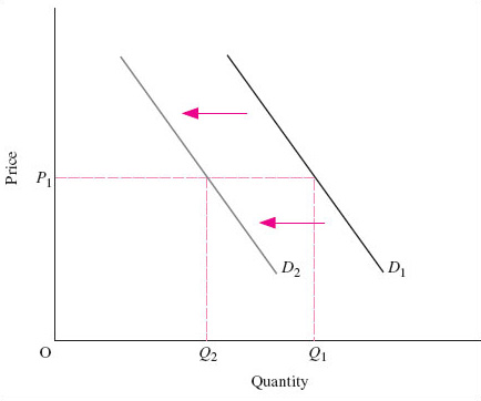
Figure 4 shows such a shift in demand. This figure does not have a numerical scale on the axes, as in Figure 3. Instead, the axes are just labelled ‘Price’ (P) and ‘Quantity’ (Q). ‘Quantity’ should be understood as ‘quantity per period of time’, such as a day, a week or a year. Diagrams such as this allow us to focus on the direction of change of variables and their implications, rather than exact magnitudes. Let us suppose that consumer incomes fall, so that everyone has less to spend on normal goods. The quantity demanded will therefore decrease at all prices. For example, at price P1 quantity demanded falls from Q1 to Q2. This means that we now have a new relationship between quantity demanded and price, and this is shown by the new market demand curve D2 in Figure 4 lying to the left of the original one, D1.
The key points about movements along and shifts of the market demand curve are:
If the price of the good changes while all other variables remain the same, this is reflected in a movement along the market demand curve.
If a variable other than the price of the good itself changes, the whole curve shifts, showing that after the change in the variable more (or less) is now demanded at each price.
Here is an exercise to help you think about shifts in the market demand curve.
Exercise 1
Think for a few minutes about how other things besides price may not remain equal in the market for electronic personal organisers. Work out what effect each will have on the demand curve. Then see if you can complete Table 1 below.
| Change in variable | Effect on demand curve |
|---|---|
| Decrease in income | Decrease in quantity demanded at all prices. Demand curve shifts to the left |
| Increase in income | |
| Rise in price of a substitute | |
| Fall in price of a substitute | |
| Rise in price of a complementary good | |
| Fall in price of a complementary good | |
| Change in socio-economic influences in favour of electronic personal organisers | |
| Change in socio-economic influences away from electronic personal organisers |
Discussion
| Change in variable | Effect on demand curve |
|---|---|
| Decrease in income | Decrease in quantity demanded at all prices |
| Demand curve shifts to the left | |
| Increase in income | Increase in quantity demanded at all prices |
| Demand curve shifts to the right | |
| Rise in price of a substitute | Demand curve shifts to the right |
| Fall in price of a substitute | Demand curve shifts to the left |
| Rise in price of a complementary good | Demand curve shifts to the left |
| Fall in price of a complementary good | Demand curve shifts to the right |
| Change in socio-economic influences in favour of electronic personal organisers | Demand curve shifts to the right |
| Change in socio-economic influences away from electronic personal organisers | Demand curve shifts to the left |