3.3 Long-run costs and economies of scale

What makes it possible to offer more output for sale at a lower price? That was one of the questions with which Section 3.2 opened. Part of the answer is that the firm's cost curves, which reflect the technology it is using, may display falling average cost as output increases over a range of output levels. The other part of the answer is that market demand must be sufficient to justify successive expansions of output. A firm such as the cable supplier seeking to increase sales by offering ‘bargain prices’ to its new customers is making an assumption about the size of the market. This section examines the relation between output and average cost on the assumption that the size of the firm's market is sufficiently large to justify increases in its input of all factors of production.

There is greater scope for cutting costs in the long run. In the long run the firm can increase inputs of all factors of production: labour, capital and land. This corresponds in reality to firms making investments. Firms invest in labour by training key personnel such as train drivers, technicians and telephonists. They may invest in items of capital equipment from telephones and computers to new factories or warehouses. They may invest in land by buying more office space or, literally, perhaps by buying a ‘greenfield’ site for a new runway. In modelling firms in the long run, it is still assumed that they are operating with given technology available to all firms.

How exactly do economists analyse the effects of investment of this kind on the firm's costs? The long-run average cost (LRAC) curve models the relationship between changes in output and average cost (AC) in the long run (Figure 6). Each point on the LRAC curve represents the average cost, in the long run, of producing a given quantity of output. The shape of the LRAC curve varies with the technology in use by firms in a particular industry. An increase in output in the long run is described as an increase in the scale of production, the phrase reflecting the implications of investment in plant and equipment. In the long run, a firm can adjust the quantities of all its factors of production to produce its desired level of output at the lowest possible cost. To achieve higher levels of output, a firm will need to buy more factors of production. How will costs change?

Figure 6: Long-run average cost (LRAC) curves. (a) LRAC curve displaying increasing, constant and decreasing returns to scale; (b) ‘L’-shaped LRAC curve; and (c) downward-sloping LRAC curve

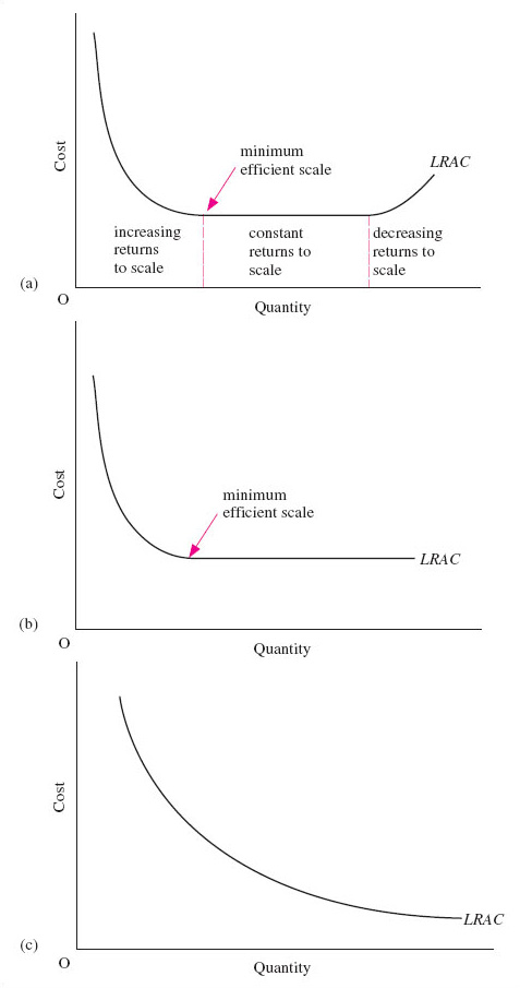
Figure 6 shows three possible shapes for the firm's long-run average cost (LRAC) curve. All three have a downward-sloping section: in (a) and (b) this occurs at low output levels; in (c) LRAC slopes down continuously over the whole output range. If the LRAC slopes downwards, the firm is benefiting from increasing returns to scale or economies of scale over the relevant range of output. We will use these two terms interchangeably. They both refer to a decrease in long-run average costs as output increases.

Increasing returns to scale arise within the firm from the firm's production function. Increased output may allow a firm to use inputs more productively. If doubling all the firm's inputs more than doubles output, there are increasing returns to scale. This may be because there are economies of increased dimensions. For example, enormous oil tankers and very large lorries can transport goods at lower cost per unit than smaller ships and vehicles because their capacity rises faster than the materials needed to make and run them. Industrial plant displays the same effect: building a factory extension that doubles the output capacity of the firm may be possible without doubling the costs of using and maintaining it. Furthermore, larger scale may also allow the more efficient use of inputs through specialisation of tasks.

The firm may also benefit from economies of scale that arise from sources outside the firm. These are reductions in a firm's average costs arising from the expansion of the industry to which it belongs. For example, the first IT firms which located in what has become known as Silicon Valley in the USA – or in Silicon Fen as the area around Cambridge, UK, is sometimes called – gained economies of scale when the industry began to expand. The concentration of numerous, closely related high-tech companies in a single geographical area meant that highly specialised factors of production (e.g. computer technicians and silicon chips) were available to them more cheaply and easily than they were to firms located elsewhere.

Firms may find that there is a limit to the economies of scale that they can achieve, a situation shown in Figure 6 (a). They will reach a level of output after which no further reductions in average cost can be obtained. This level of output is known as the minimum efficient scale (MES). The MES marks the size of the firm beyond which there are no cost advantages to be reaped from operating at a larger scale, or the output at which long-run average costs first reach their minimum level as output rises. In other words, it is the point at which all economies of scale have been taken up. As Henry Ford's smaller rivals discovered, once large-scale assembly-line production had been developed serious cost disadvantages were incurred by a firm operating below the MES, where average cost is higher than it would be if all scale economies were to be exploited. The MES is located at the beginning of the flat section of the LRAC curve, over which average cost is constant in Figure 6 (a). The firm is experiencing constant returns to scale over this range of output. Constant returns to scale exist when long-run average cost remains unchanged as output increases.

The LRAC curve depicted in Figure 6 (a) rises at high levels of output. Average costs increase as output increases. The firm is now experiencing decreasing returns to scale or diseconomies of scale. Decreasing returns to scale or diseconomies of scale exist when long-run average cost rises as output increases and arise from the disadvantages that large-scale production may entail. The major source of diseconomies of scale is the co-ordination problems that beset management in large bureaucratic organisations. The rapid expansion of an industry may also cause external diseconomies of scale, if labour costs increase as more and more firms chase scarce supplies of specific skills. For example, firms in some ‘new economy’ industries find wages are being bid up because of a shortage of workers with the appropriate IT skills.

The ‘U’-shaped LRAC curve shown in Figure 6 (a) is only one of three possible shapes that are usually distinguished. If the technology of the industry in which the firm is active is different from that of another industry, this will be expressed in a different LRAC curve. In Figure 6 (b) the LRAC curve is ‘L’-shaped, indicating that the firm continues to experience constant returns to scale across its output range once output is above the MES. This might correspond to a firm that can continue to replicate its production processes, for example by adding additional assembly lines, each one exactly like the others.

A third possibility is depicted in Figure 6 (c), where the firm enjoys economies of scale right across its output range. There is, therefore, every incentive, in the form of ever lower average costs, for firms to continue to expand output. A single firm can supply the whole market at a lower cost than could be achieved by a number of firms in competition with each other. Network industries such as gas, water and electricity distribution, fuel retailing, railway track and cable networks in telecommunications are examples of industries where firms are appropriately modelled by the LRAC curve shown in Figure 6 (c).

The three LRAC curves in Figure 6, considered together, imply that the technology of an industry is expressed in the shape of the particular LRAC curve used in modelling that industry. There is a further implication, which is that technology, reflected in costs, shapes the structure of the industry. If, for the moment, the ‘structure’ of an industry is understood to mean the number and size of firms that are active in it, this point can be illustrated in a number of ways. You have already seen that the US automobile and PC industries experienced a ‘shake-out’ of small firms as product standardisation enabled the exploitation of economies of scale.

In industries in which firms experience constant returns to scale there will be a minimum level of output, the MES, at which constant returns set in, that firms must be able to sustain if they are to remain competitive. The MES varies with the particular technologies characteristic of different industries. For many parts of the clothing, footwear and furniture industries, all economies of scale may be exploited at relatively low levels of output and so the MES is low relative to market size. By contrast, in industries such as automobiles and chemicals where economies of scale are available over much greater ranges of output, the MES is much higher in relation to the size of the market.

The existence in some industries of a level of output beyond which decreasing returns are experienced sets a limit to the size of firms and hence to the pressure for mergers and acquisitions. In fact, decreasing returns to scale can lead to the break-up of very large firms so that management can focus on making the ‘core’ business more competitive. The break-up of the chemicals firm ICI into ICI and Zeneca in 1993 can be interpreted as an example of this kind of behaviour.

If increasing returns are available across the whole output range required to supply the market, this has dramatic implications for industry structure. A single producer can supply the entire market at a lower cost than two or more competing firms. This is because a single firm avoids the cost of duplicating distribution networks such as gas, water and electricity pipes, railway track and telecommunications cables.

The technology of an industry, expressed in the shape of the LRAC curve of its firms, is therefore a major influence on the structure of that industry. However, in modelling firms’ costs in the short run and the long run, it has been assumed that firms are operating with given technology. It is now appropriate to relax this assumption and investigate the role of technological change in shaping industrial structure.

As Section 3.2 explained, a firm's production function embodies its technology. The model assumes that technology is given and is available to all firms in an industry. We can therefore think of technological change as a change in each firm's production function. Particular input combinations now become more productive, producing more output. What effect does this have on the long-run average cost curve?

Figure 7: A downward shift in the LRAC curve

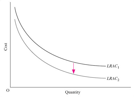
The LRAC curves in Figure 6 were drawn on the assumption of given technology. Technological change can therefore be understood as a shift in the average cost curve. Figure 7 shows a downward shift in an LRAC curve like that shown in Figure 6 (c). The shift of LRAC₁ downward to LRAC₂ in Figure 7 shows that long-run average costs have fallen at each and every level of output, or scale of production.

Technological change may not affect average costs at all levels of output. Henry Ford's introduction of moving assembly-line production methods is an example of a technological change that changed the shape of the LRAC curve for firms in the industry, shifting it downwards at high levels of output. The new methods hugely extended the range of output over which firms could benefit from increasing returns to scale. In this way, technological change, and its associated cost changes, exert a major influence on industrial structure. We explore this further in Section 4.