2.4 First-order filters

In addition to the filter categories already introduced (low-pass, band-pass, etc.), filters are categorised by their order. The order of a filter is determined by the form of the differential equation governing the filter’s behaviour. The simplest type of filter, with the simplest equation, is called a first-order filter. Higher-order filters are more complex than first-order filters, both in their circuitry and in the differential equation that governs them. The higher the order, the more effective the filter.

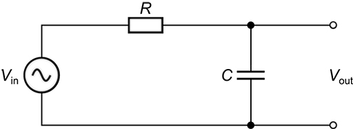
An example of a first-order filter is the simple circuit in Figure 8.

Figure 8 First-order filter

Show description|Hide description

This figure is a circuit diagram in which the input voltage, V subscript in, is produced by an alternating source. The source is in series with a resistor, R, and a capacitor, C. The output voltage, V subscript out, is taken across the capacitor.

Figure 8 First-order filter

Activity 3

Timing: Allow about 5 minutes

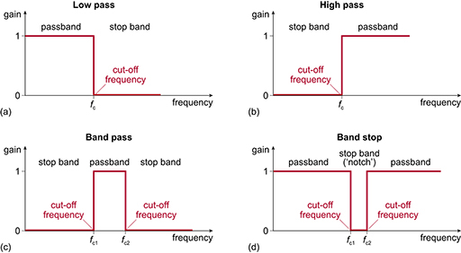
Which of the four categories of filter shown in Figure 5 does the filter in Figure 8 belong to? You should be able to work it out from the behaviour of the capacitor at low frequencies and high frequencies. Explain your answer.

Figure 5 (repeated) Four types of ideal filter: (a) low-pass filter; (b) high-pass filter; (c) band-pass filter; (d) band-stop (notch) filter

Show description|Hide description

This figure consists of four graphs of gain against frequency, representing four types of filter. In each case, the gain is either at 1 or at 0, depending on the frequency. Areas where the gain is 1 are labelled ‘passband’, while areas where the gain is 0 are labelled ‘stop band’. The transitions between 1 and 0 (or vice versa) are vertical, and labelled ‘cut-off frequency’.

Part (a) is a low-pass filter. There is a single cut-off frequency, f subscript c. At frequencies below the cut-off, the gain is 1 (passband). At frequencies above the cut-off, the gain is 0 (stop band).

Part (b) is a high-pass filter. There is a single cut-off frequency, f subscript c. At frequencies below the cut-off, the gain is 0 (stop band). At frequencies above the cut-off, the gain is 1 (passband).

Part (c) is a band-pass filter. There are two cut-off frequencies, f subscript c1 and f subscript c2. At frequencies below f subscript c1 and above f subscript c2, the gain is 0 (stop band). At frequencies between f subscript c1 and f subscript c2, the gain is 1 (passband).

Part (d) is a band-stop filter. There are two cut-off frequencies, f subscript c1 and f subscript c2. At frequencies below f subscript c1 and above f subscript c2, the gain is 1 (passband). At frequencies between f subscript c1 and f subscript c2, the gain is 0 (stop band). Because the stop band is a narrow region between two passbands, the stop band is also known as the notch in this type of filter.

Figure 5 (repeated) Four types of ideal filter: (a) low-pass filter; (b) high-pass filter; (c) band-pass filter; (d) band-stop (notch) ...

Answer

It is a low-pass filter.

At 0 Hz, or DC, the capacitor is open circuit. Under those circumstances, all the input voltage would appear on the output. At high frequencies, the capacitor becomes increasingly like a short circuit, and the output voltage decreases as frequency increases. Therefore low frequencies are passed and high frequencies are (to some extent) blocked.

Low-pass and high-pass filters can be first-order, second-order, third-order, and so on. However, band-pass filters and band-stop filters must be second-order or higher, although it is possible to achieve their effect by combining two first-order filters.

Despite being the simplest type, a first-order filter is not simple to analyse mathematically, as its behaviour is governed by a first-order differential equation. This is what the voltage gain function of the filter in Figure 8 turns out to be:

You could plot a graph of the gain function against frequency from this equation, but the details would depend on the choice of and . However, irrespective of the values chosen for and , the general shape and certain other properties of the gain function would be the same for any first-order low-pass filter. Therefore, rather than show how the gain function changes with frequency for particular values of and , in the next section you will look at a ‘normalised’ version of the gain function. (Normalisation is the presentation of information in a generalised way that can easily be adapted to specific cases.)