3.6 Designing a digital filter in the frequency domain

Most digital filters are designed in the frequency domain. Input signals are characterised by their frequency spectrum and design filters to modify that spectrum by, for example, removing high-frequency noise with a low-pass filter.

Figure 22 shows the four basic filter structures in the frequency domain. These ideal filters are identical for both analogue and digital filters (you have already seen them earlier in the course in Section 2.2).

Figure 22  Ideal filter responses: (a) low-pass; (b) high-pass; (c) band-pass; (d) band-stop (repeat of Figure 5)

Show description|Hide description

This figure consists of four graphs of gain against frequency, representing four types of filter. In each case, the gain is either at 1 or at 0, depending on the frequency. Areas where the gain is 1 are labelled ‘passband’, while areas where the gain is 0 are labelled ‘stop band’. The transitions between 1 and 0 (or vice versa) are vertical, and labelled ‘cut-off frequency’.

Part (a) is a low-pass filter. There is a single cut-off frequency, f subscript c. At frequencies below the cut-off, the gain is 1 (passband). At frequencies above the cut-off, the gain is 0 (stop band).

Part (b) is a high-pass filter. There is a single cut-off frequency, f subscript c. At frequencies below the cut-off, the gain is 0 (stop band). At frequencies above the cut-off, the gain is 1 (passband).

Part (c) is a band-pass filter. There are two cut-off frequencies, f subscript c1 and f subscript c2. At frequencies below f subscript c1 and above f subscript c2, the gain is 0 (stop band). At frequencies between f subscript c1 and f subscript c2, the gain is 1 (passband).

Part (d) is a band-stop filter. There are two cut-off frequencies, f subscript c1 and f subscript c2. At frequencies below f subscript c1 and above f subscript c2, the gain is 1 (passband). At frequencies between f subscript c1 and f subscript c2, the gain is 0 (stop band). Because the stop band is a narrow region between two passbands, the stop band is also known as the notch in this type of filter.

Figure 22  Ideal filter responses: (a) low-pass; (b) high-pass; (c) band-pass; (d) band-stop (repeat of Figure 5)...

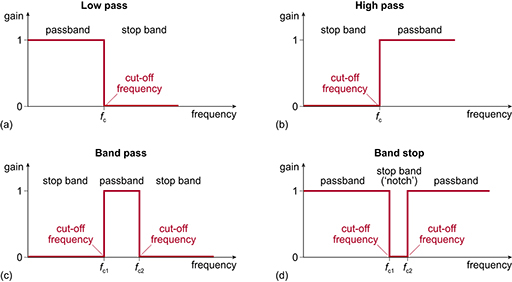
In the design process, the aim is to produce a filter frequency response that best matches the profile of the filter; however, compromises have to be made. You have already seen how the order of the design of the filter affects the roll-off, so decisions are made in the design of these analogue filters to best match the filter to the ideal response.

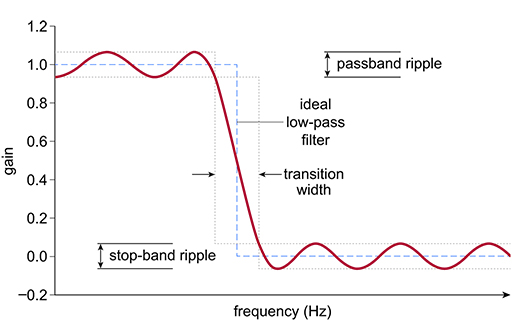
Figure 23 shows some of the characteristics of a typical low-pass digital filter. In comparison to the ideal shape (shown in red), there is a transition region between the passband and stop-band sections, and also a ripple in both the passband and the stop band. These effects can be altered by changing various parameters in the design.

Figure 23 Typical low-pass digital filter response

Show description|Hide description

This figure is a graph of gain against frequency. An ideal low-pass filter line is shown that is horizontal at a gain of 1 for low frequency values, then falls vertically at the cut-off frequency and remains horizontal at a gain of 0 for frequency values above this point. Another line is shown representing the actual response of the digital filter. At low frequencies, it oscillates by a small amount around a gain of 1; this is known as the passband ripple. At a frequency slightly below the cut-off, it descends diagonally until it reaches a frequency slightly above the cut-off; the distance between these two frequency values is known as the transition width. At frequencies above this, the response oscillates by a small amount around a gain of 0; this is known as the stop-band ripple.

Figure 23 Typical low-pass digital filter response

When designing a digital filter in the frequency domain, software tools are most often used to generate the mathematical expression for the filter. This expression is in the form of a difference equation – an equation involving combinations of samples at specific times. You have already seen a difference equation in this section: the equation   =  for the three-term averaging filter. As another example, the following difference equation contains five terms:

In a digital filter design, the number of terms in the difference equation is often referred to as the number of taps, and is specified as a design parameter. A larger number of taps may give a filter design that more closely matches the desired specification; however, more taps will mean that it takes longer to compute the filter outputs.

There are two main classes of LTI (linear time-invariant) digital filter: the finite impulse response (FIR) filter and the infinite impulse response (IIR) filter. An IIR filter requires fewer computations to achieve the same performance as an FIR filter, so has a speed advantage. However, an IIR can have stability issues and also non-linear phase issues (where signals of different frequencies are delayed by different amounts, resulting in a distortion of the output signal). The difference between an FIR filter and an IIR filter is that the FIR filter uses only the filter inputs when generating its output, whereas an IIR filter uses both the filter inputs and past filter outputs – in other words, it uses feedback. The difference equation above is for an FIR filter. The difference equation below has four terms and the final term is an output value, so it is an IIR filter:

To calculate the output of an IIR filter, both previous input samples and previous output samples are stored in the processor’s memory. The order of the IIR filter is the larger of the number of input values stored and the number of output values stored. In the above example, the filter is second-order, since two previous input values are stored but only one previous output value.

Before you look at a filter being designed, you need to know a little more about the relationship between the time domain and the frequency domain. You will cover this next.