3.9 Digital filtering in practice

You are now going to use an interactive resource to add Gaussian noise to a noise-free (or ‘clean’) data signal. The noisy data signal is passed to a detector, which determines whether received samples are binary zeros or ones. The added noise causes the detector to make mistakes; hence there are bit errors. Using a finite impulse response (FIR) digital filter, you will ‘clean up’ the noisy data signal and thereby reduce the bit-error rate.

Right-click on the image or link below to open Interactive 1 in a new tab or window so you can continue to work through the course and activities with the interactive alongside. The interface consists of four equally sized zones: top left, top right, bottom left and bottom right. Note that depending on the browser you are using, the sliders and other components in the interface may have a different visual appearance from those shown in the screenshots in this document, but the functionality will be the same.

View interactive version

Interactive 1 FIR filter

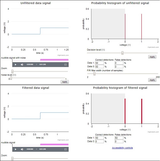
The top left zone shows the signal, whether it is clean or noisy. When the interactive resource is launched, the noise level is at zero and the signal is clean. The data signal is shown as a single step from 0 to 1, but there are 10 000 samples for this data signal, half of which are from the 0 part of the signal and half of which are from the 1 part. Noise is added by sliding the Noise level (V) slider to the right and clicking on Apply.

The top right zone displays a histogram of the signal. As there is an equal number of zeros and ones in the signal, the probability of each is 0.5. The detected probabilities of zeros and ones in the received signal are shown by the vertical red lines situated at 0 and 1. Without added noise, perfect detection can be achieved.

The top right zone allows the decision level at the detector to be set using the Decision level (V) slider, and also the degree of low-pass filtering to be set using the FIR filter width (number of samples) slider. Finally, the top right zone also gives statistics about the number of true and false detections. Figure 32 explains how to interpret this data. Before noise is added, all samples are correctly identified, so False detections should be at 0 to start with.

Figure 32 Interpreting the statistics

Show description|Hide description

This figure shows the four fields from the interactive interface that contain statistics about the number of true and false detections. They are arranged in a two by two grid, with the rows labelled Data 1 and Data 0, and the columns labelled Correct detections and False detections. The four possible combinations of these row and column values have the following meanings.

• Data 1, Correct detections: samples correctly identified as 1, as a percentage of all samples. Shown as 50 per cent in this example.
• Data 0, Correct detections: samples correctly identified as 0, as a percentage of all samples. Shown as 50 per cent in this example.
• Data 1, False detections: samples originally 0 but incorrectly identified as 1. Shown as 0 per cent in this example.
• Data 0, False detections: samples originally 1 but incorrectly identified as 0. Shown as 0 per cent in this example.

Figure 32 Interpreting the statistics

Note in Figure 32 that if the correct detection of data 1s were to drop below 50%, the deficit would appear as an increase in the false detection of data 0s. Similarly, if the correct detection of data 0s drops below 50%, the deficit should appear as an increase in the false detection of data 1s. Thus the diagonal pairs of statistics in Figure 32 should always add up to 50% – or approximately 50%, given the possibility of rounding errors in the calculation.

The bottom left zone shows the effect of filtering applied to a noisy signal. The bottom right zone is similar to the top right zone, showing a signal histogram and false detection statistics; however, these are after filtering, whereas the top right zone is before filtering.

In the next section you will have a go at adding noise to the data signal in the interactive.