
Export Supply (25 minute read)
Learning Outcome:
After completing this lesson, you will understand how export supply is described by a constant-elasticity of transformation (CET) function in the UNI-CGE model, and the role of the CET elasticity in producer decision-making.
Producer Problem - Where to Sell their Output?
Many producers make commodities that can be either sold in the domestic market or exported to foreign markets. How do they decide which market in which to sell their output? Some CGE models, including the UNI-CGE model, describe this decision using a constant elasticity of transformation (CET) export supply equation. It describes how easily producers can transform their product to be suitable for sale in the export or domestic market.
The insight of the CET function is the same as that of the Armington CES import demand function: different varieties of the same product are differentiated in some way. A producer's output is a "composite" good made up of the variety sold domestically and the exported variety. For example, the commodity "chocolate bars" may be made with less cocoa butter for the domestic market and more of that ingredient for foreign markets. Because the chocolate bars are differentiated by their destination market, their prices can be different, too.
Producers maximize their profits by shifting their sales to the market in which the relative price is higher - to the extent their production process is flexible enough to allow this. The ease with which a producer can transform their product across the two market is described by an elasticity of transformation. This parameter is named ETRAX in the UNI-CGE model (Elasticiticy of TRAnsformation of eXports), and it is expressed as a negative number. When its absolute value is high, it is relatively easy to shift the production line between the two varieties in response to relative price changes. When the parameter's absolute value is low, the product transformation between the two varieties is more costly, and the quantity response of export supply is more limited.
Export Transformation Decision - A Graphical View
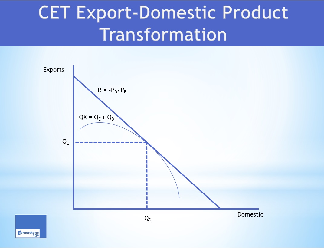
Figure 1 depicts the producer's product transformation decision. In the figure, curve QX is an isoquant that shows all combinations of the variety sold domestically (QD) and exported (QE) that make up the same composite quantity of output. The further is QX from the origin, the larger the quantity of commodity output. As the producer moves down the isoquant, exports account for a large quantity share in the total output of QX. Line R is an isorevenue line with a slope of -PD/PE, where PD is the price of the domestically-sold variety and PE is the price of the exported variety. Line R shows all combinations of domestic and export sales that generate the same level of revenue. The further R lies from the origin, the higher is the revenue earned by the producer. The producer gets the highest achievable revenue for a given level of output by choosing the product ratio shown at the tangency between the isoquant and the highest achievable isorevenue line. In Figure 1, the optimal quantities of domestic and export sales are QD and QE, respectively.
Figure 1. CET Production Transformation Decision
Larger version of figure is available HERE
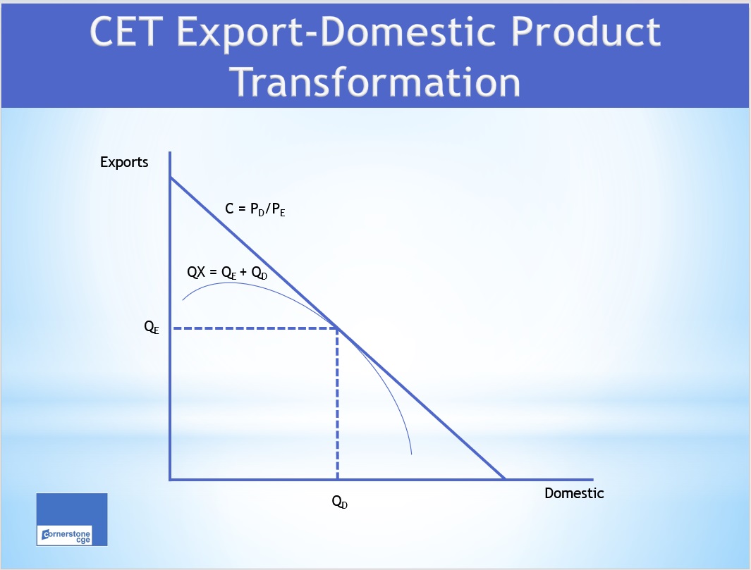
Figure 2 describes the effects of a change in relative prices on the ratio of the two varieties in an activity's output. In the figure, the price of exports increases relative to the domestic sales price, as shown by the rotation of the isorevenue line to price ratio PD'/PE' (shown in red). This price shock may be due to an increase in the world price, or a new subsidy on exports. Holding total output constant, by remaining on isoquant QX, the producer shifts production toward a greater share of exports in the product mix. In the new equilibrium, the producer now makes quantities QE' and QD'.
Figure 2. CET Export-Domestic Ratio with a Price Change
Larger figure available HERE.
The magnitude of the shift in the producer's output mix depends on the curvature of the isoquant. The degree of curvature is determined by the elasticity of transformation. When the absolute value of the parameter value is low, the curve is more concave. The varieties are not easily transformable, so the quantity response to a change in relative prices is limited. The higher the parameter's absolute value, the flatter is the isoquant - the same rotation in the isorevenue line will lead to a larger change in the QE/QD quantity ratio in output of QX. This larger quantity response in turn leads to larger economy-wide impacts than would occur with a low ETRAX parameter value.
Export Supply in the UNI-CGE Model
The UNI-CGE model includes two equations to describe export supply. The first is the CET transformation function, written in Figure 3 and shown as the isoquants in figures 1 and 2. It describes the producer's flexibility to shift between exported and domestic varieties in total output. In the equation, QXc is the quantity of composite commodity c, which is composed of quantities of the exported variety (QEc) and the variety sold domestically (QDc). Parameter alphaxc is a shift parameter calculated during the model calibration. The deltaxc parameter is the share of exports in the quantity of the composite commodity output, and 1-delta is the share sold domestically. The exponent term rhoxc is a transformation of the CET export supply elasticity, ETRAX. Parameter rhoxc is calculated for each commodity c as:
rhoxc = (1 / ETRAXc) + 1

Larger version available HERE.
The first order condition describes the quantity shares of the export/domestic varieties in total output of a commodity. It defines the quantity ratio as a function of the varieties' relative prices, PE/PD, the initial shares, and the transformation elasticity. When the relative price of the exported variety increases, its quantity share in the output mix increases - and vice versa.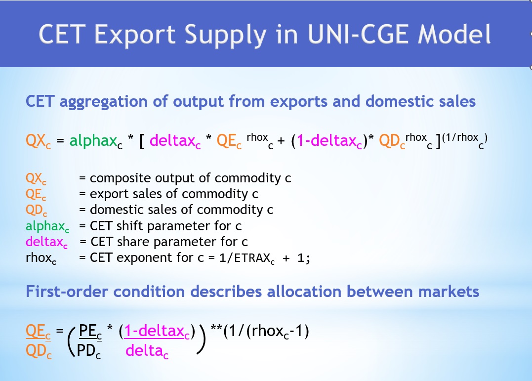
CHECK YOUR UNDERSTANDING
Copyright: CC 4.0 BY-NC-SA