
Investment Demand (18 minute read)
Learning outcome:
At the end of this lesson, you will understand and be able to explain investment demand behavior in the UNI-CGE model.
Investment Spending in the SAM
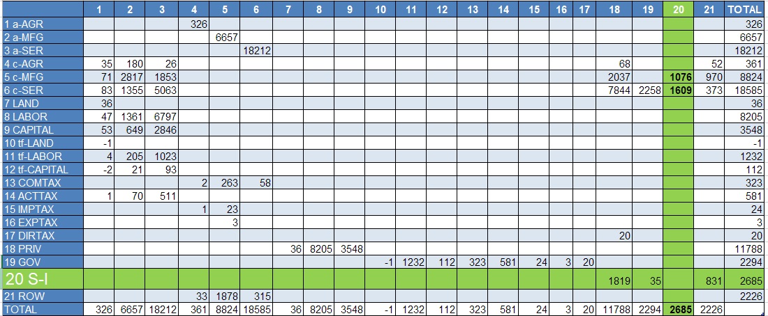
The Savings-Investment row and column in the SAM describe the sources of savings and report how investors spend those savings on goods and services.
In the US333 SAM, the savings-investment row and column are shaded in green (Table 1). The S-I row reports the total supply of savings that is available to investors. Households save $1,819 billion, the government saves $35 billion (which is a government fiscal surplus) and foreign capital inflows total $831 billion. The total supply of savings, from domestic and foreign sources, is $2,685 billion.
The savings-investment column (column number 20) shows how U.S. investors spend those savings. They purchase $1,078 billion worth of manufactured goods, and $1,609 billion worth of services.
The column total of the S-I is "gross" investment. What is "net" investment? Some SAMs report that the capital factor's column account contributes to the S-I row. This cell (which is empty in the US333 SAM) measures depreciation, or the wearing out of capital equipment. It is the money spent by firms on replacement costs. Net investment is calculated as gross investment minus depreciation. The concept takes into account that some investment spending does not add to the capital stock, it merely replaces worn-out equipment. If you want to measure investment spending, use the figure for gross investment. If you want to measure the addition to the national stock of capital, calculate net investment spending.
Table 1. Savings-investment accounts in the US333 SAM
View a large type version of Table 1 HERE.
Investment Demand in the UNI-CGE Model - Fixed Quantity Shares
Investors in the UNI-CGE model are assumed to have a simple demand function. The quantity shares of each commodity in their initial investment spending, as reported in the SAM, always remain the same. Why does the model have such a simple depiction of an important part of the economy? CGE models are "real" models - they do not include monetary policy and interest rates, which are the main drivers of investment decisions. And, the UNI-CGE model does not include expectations about the future, another key driver of investment decisions. Maintaining fixed quantity shares is simple and transparent, and reflects the investment decisions that have been observed in the past.
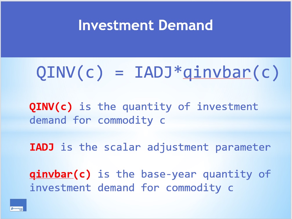
The investment demand equation in the UNI-CGE model, presented in Figure 2, is almost identical to that of government demand. The variable QINVc is the quantity of investment spending on each commodity. Variable IADJ is a scalar whose initial value is one. Parameter invbarc is the quantity of each commodity initially purchased by investors and reported in the SAM.
Figure 2. Investment demand function in the UNI-CGE model
How do investors behave if the supply of savings changes, or if the prices of investment goods change? It depends on the savings-investment closure that you have selected (see the lesson on macro closures in the Macro and GE module). Either the supply of savings or the quantities of goods must change to maintain an equivalence between savings and investment.
Closure 1 - Fixed Supply of Savings
If the closure fixes the supply of savings, then investment spending must change to accommodate it. For example, if the prices of one or more investment goods changes, the value of investment spending would also change. Rather than under- or overspend relative to the fixed amount of available savings, the quantity purchased of investment goods (QINV) must change. Variable IADJ will adjust all initial quantities (qinvbar) by the same proportion, maintaining commodities' fixed quantity shares in the investment basket, until savings is again equal to investment spending.
Closure 2 - Fixed Investment Spending
If the closure instead fixes investment spending, then the supply of savings must adjust to accommodate any changes in investment spending. In this case, variable IADJ remains fixed at the value of one so investors' purchases of each commodity always remains at initial levels (qinvbar). If commodity prices change, the cost of investment purchases will change. In this case, the savings rate will change until the supply of savings is equal to the new level of investment spending.
CHECK YOUR UNDERSTANDING
Copyright Cornerstone CC 4.0 BY-NC-SA