

3.3 The projective plane
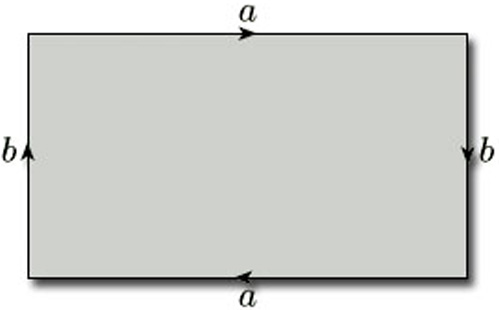
We now consider one of the most important non-orientable surfaces – the projective plane (sometimes called the real projective plane). In Section 2 we introduced it as the surface obtained from a rectangle by identifying each pair of opposite edges in opposite directions, as shown in Figure 61. The projective plane is of particular importance in relation to the classification of surfaces – the Classification Theorem can be interpreted as saying that all surfaces without boundary can made from a sphere by adjoining either toruses or projective planes.
You may already be familiar with a geometric way of viewing the projective plane. This gives a completely different way of thinking about it: indeed, it is not even immediately obvious from the geometric approach why it is a surface!
The geometric approach is to define the projective plane as the set of all infinite lines through the origin in Euclidean three-dimensional space: this means that each infinite line through the origin is to be regarded as a ‘point’ of the projective plane. To do this, we take ![]() 3, remove the origin (0, 0, 0), and consider any two of the remaining points (x, y, z) and (x', y', z') of
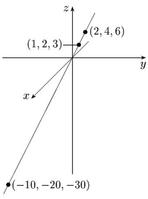
3, remove the origin (0, 0, 0), and consider any two of the remaining points (x, y, z) and (x', y', z') of ![]() 3 to be equivalent if and only if they lie on the same infinite line through the origin – that is, x' = kx, y' = ky, z' = kz, for some non-zero real number k. For example, the points (1, 2, 3), (2, 4, 6) and (−10, −20, −30) of
3 to be equivalent if and only if they lie on the same infinite line through the origin – that is, x' = kx, y' = ky, z' = kz, for some non-zero real number k. For example, the points (1, 2, 3), (2, 4, 6) and (−10, −20, −30) of ![]() 3 are all equivalent points, as Figure 62 illustrates. Each set of equivalent points, together with the point (0, 0, 0), comprises an infinite line through the origin and is thus a ‘point’ of the projective plane, which we refer to as a projective point. We denote a projective point using square brackets around the coordinates of a representative point on the infinite line: thus the projective point containing the points (1, 2, 3), (2, 4, 6) and (−10, −20, −30) may be written as [1, 2, 3] or [2, 4, 6] or indeed as [k, 2k, 3k] for any non-zero number k.
3 are all equivalent points, as Figure 62 illustrates. Each set of equivalent points, together with the point (0, 0, 0), comprises an infinite line through the origin and is thus a ‘point’ of the projective plane, which we refer to as a projective point. We denote a projective point using square brackets around the coordinates of a representative point on the infinite line: thus the projective point containing the points (1, 2, 3), (2, 4, 6) and (−10, −20, −30) may be written as [1, 2, 3] or [2, 4, 6] or indeed as [k, 2k, 3k] for any non-zero number k.
Problem 15
Which of the following points (x, y, z) of ![]() 3 correspond to the same projective points [x, y, z]?
3 correspond to the same projective points [x, y, z]?
(3, −1, 2), (4, −2, 6), (−9, 3, −6), (12, −6, −9), (15, −5, 10), (−18, 9, −27).
Answer
(3, −1, 2), (−9, 3, −6) and (15, −5, 10) correspond to the projective point [3, −1, 2]. (4, −2, 6) and (−18, 9, −27) correspond to the projective point [4, −2, 6] = [2, −1, 3]. (12, −6, −9) corresponds to the projective point [12, −6, −9] = [4, −2, −3].
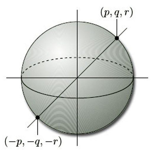
This definition of the projective plane is no more helpful than the definition in terms of a rectangle with edge identifications as a means of picturing what the projective plane really looks like. It does, however, lead us towards a description of the projective plane in which each projective point looks like a point of ![]() 3. We begin by enclosing the origin within the sphere of unit radius, as shown in Figure 63. Each infinite line through the origin gives rise to a diameter of this sphere which meets the sphere in exactly two antipodal points, (p, q, r) and (−p, −q, −r). So we can think of the projective plane as the set of all these pairs of antipodal points on the unit sphere, and the projective point [p, q, r] now corresponds to the two points (p, q, r) and (−p, −q, −r) of
3. We begin by enclosing the origin within the sphere of unit radius, as shown in Figure 63. Each infinite line through the origin gives rise to a diameter of this sphere which meets the sphere in exactly two antipodal points, (p, q, r) and (−p, −q, −r). So we can think of the projective plane as the set of all these pairs of antipodal points on the unit sphere, and the projective point [p, q, r] now corresponds to the two points (p, q, r) and (−p, −q, −r) of ![]() 3 on the sphere. This gives a natural ‘two-to-one’ map from the sphere to the projective plane which sends the two points (p, q, r) and (−p, −q, −r) to the projective point [p, q, r].
3 on the sphere. This gives a natural ‘two-to-one’ map from the sphere to the projective plane which sends the two points (p, q, r) and (−p, −q, −r) to the projective point [p, q, r].
This sphere has equation![]()
So we can regard the projective plane as made up of pairs of points on the sphere. If we could systematically select a single point from each of these pairs, then we would have an even better picture of the projective plane. Unfortunately, there is no natural way of thinking of exactly half of the points on a sphere. We can certainly think of the points [p, q, r] with r ≠ 0 as lying on the upper hemisphere: we simply associate with each projective point [p, q, r] whichever of the two points (p, q, r) and (−p, −q, −r) on the sphere has its third coordinate positive. But if r = 0 then we have a problem: the projective point [p, q, r] is associated with both the points (p, q, 0) and (−p, −q, −0) of the sphere, and there is no satisfactory way of choosing just one of them.
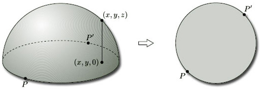
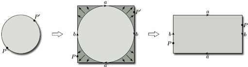
Instead, we proceed as follows. We first represent the projective plane as the upper hemisphere with antipodal pairs of points on the equator (r = 0) identified. We then map this space on to the unit disc by projecting vertically downwards, using the map (x, y, z) ![]() (x, y, 0), as shown in Figure 64. We thereby represent the projective plane as a disc with antipodal points P and P' on the boundary identified.
(x, y, 0), as shown in Figure 64. We thereby represent the projective plane as a disc with antipodal points P and P' on the boundary identified.
Finally, we project this disc radially onto a circumscribing square. This represents the projective plane as a square with diagonally opposite points P and P' on the boundary identified, as shown in Figure 65. By stretching the square to a rectangle, we obtain our earlier description of the projective plane as a rectangle with opposite edges identified in opposite directions.
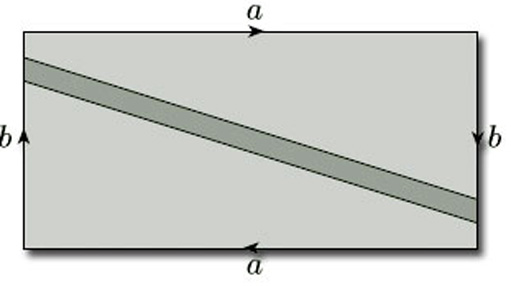
In Section 3.2 we asserted that a surface is non-orientable if it contains a Möbius band. To show that the projective plane is non-orientable, we consider its representation as a rectangle with opposite edges identified in opposite directions, as shown in Figure 66. When we identify the edges labelled b, the shaded strip becomes a Möbius band. This shows that the projective plane contains a Möbius band, and therefore by Theorem 4 is non-orientable.
Problem 16
Use the Klein bottle's representation as a rectangle with edge identifications (see Figure 31) to show that it is non-orientable.
Answer
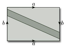
The Klein bottle's representation as a rectangle with edge identifications is shown below. When we identify the edges labelled b, the shaded strip becomes a Möbius band, and thus by Theorem 4 the Klein bottle is non-orientable.
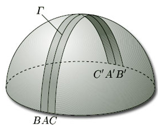
We can obtain the same result using the representation of the projective plane as an upper hemisphere with antipodal points identified. To do so, we draw half of a great circle Γ on it through two antipodal points A, A' and the north pole. We then ‘fatten’ this line to a narrow strip that meets the equator at the pairs of antipodal points B, B' and C, C', as shown in Figure 67. The boundary of this strip around Γ is a single curve, and the shaded strip is a Möbius band, showing that the surface is non-orientable. Either way, the presence of a Möbius band shows that the projective plane is non-orientable. This result is so important that we state it as a theorem.
Theorem 5
The projective plane is non-orientable.
If we remove a Möbius band from the projective plane, what remains? Using the rectangle representation, we first obtain two pieces, as shown in Figure 68(a), with the edges labelled a, b and c to be identified in pairs; the edges x and y form the boundary of the removed Möbius band. Turning each piece over and identifying the edges labelled a, we obtain Figure 68(b). Identifying the edges labelled b and then the edges labelled c, we obtain a purse-like object whose boundary is the boundary of the Möbius band, as shown in Figure 68(c). Finally, if we open the purse and flatten it out, we obtain a disc whose boundary is the boundary of the Möbius band, as shown in Figure 68(d).
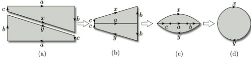
Thus, removing a Möbius band from the projective plane yields a disc whose boundary is the boundary of the Möbius band. Gluing the Möbius band back again leads to the following surprising conclusion.
Theorem 6
The projective plane is obtained by gluing a disc and a Möbius band along their boundaries.
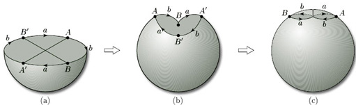
We can use this result to provide us with an alternative picture of a Möbius band. We begin with a representation of the projective plane as a hemisphere. However, instead of taking the upper hemisphere as before, it is now more convenient to represent it as the lower hemisphere, but again with antipodal points on the equation identified, as shown in Figure 69(a). We then distort the hemisphere slightly, giving the equator a ‘flower’ shape, as shown in Figure 69(b): this makes it easier for us to see what is to be identified with what. We see that the edge AB is to be identified with the edge A'B', and that the edge BA' is to be identified with the edge B'A. We can perform either one of these two identifications without too much difficulty after some judicious stretching of the surface; but, when we try to perform the other, we need to let the surface ‘intersect itself along a line, the vertical line in Figure 69(c).
Thus Figure 69(c) gives us a representation of the projective plane in which no identifications need to be made, but it is not a representation in ![]() 3 since the surface pictured intersects itself.
3 since the surface pictured intersects itself.
We saw a similar picture of the Klein bottle, as a surface that intersects itself, in Figure 31.
If we now remove a disc from the surface in Figure 69(c), as shown in Figure 70, Theorem 4 tells us that what we have left is a Möbius band. This new picture of a Möbius band is called a cross-cap, from its supposed resemblance to a bishop's mitre.
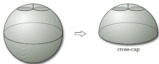
In general, we add a cross-cap to a surface by removing a disc and identifying opposite points on the boundary (or by identifying the boundary curve with that of a Möbius band). Adding one cross-cap to the sphere gives the projective plane; adding two cross-caps to the sphere gives the Klein bottle.
We stated in Section 2 that neither the projective plane nor the Klein bottle are surfaces in space. In both cases, whenever all identifications are made, the resulting representation is a surface that intersects itself and so cannot be embedded in ![]() 3. In fact, a non-orientable surface can be represented as a surface in space if and only if it has a boundary.
3. In fact, a non-orientable surface can be represented as a surface in space if and only if it has a boundary.
Theorem 7
A non-orientable surface can be represented as a surface in space if and only if it has a boundary.
(We omit the proof, which is beyond the scope of this course.)
We also have the following result:
Theorem 8
All orientable surfaces can be represented as surfaces in space.
(We omit the proof, which is beyond the scope of this course.)
So the extra freedom that we gain by studying surfaces in general, and not just surfaces in space, is precisely the freedom to study non-orientable surfaces without boundary, of which the projective plane and the Klein bottle are the most important examples.